CS 479 : AGBO Classification
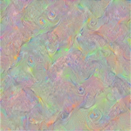
MEL Spectogram of Biophony
Introduction
Our team focused on the goal of classifying anthrophony, geophony, biophony, and other sounds (AGBO) into 4 distinct categories. Our features were png images of MEL spectrograms of a couple seconds long each. These sounds ranged from birds chirping to planes flying over the audio recording devices.
The dataset we were given was that of only a couple thousand images disproportionally set between the four categories, consisting of a variety of images that a model needed to differentiate between. An airplane was in the same category as a person talking. A bird's chirping had to be categorized alongside a dog's howl.
Approach/Algorithm
While at first the team simply fed the data into the models, we later made a concerned effort to balance the representation of the data within the data set. We implemented the randomized oversampling of underrepresented data sets. The category "other" that only had a few hundred images was duplicated randomly to a set of 3,086 images to match the largest data set of biophony. Afterwards we saw on average a few percentage points better on all of our models, with some categories like geophony and other having drastically different accuracy ratings than before.
Without Oversampling
With Oversampling
Our team was supplied with only a couple thousand images, meaning that creating our own CNN to properly classify images was out of the question. We instead relied on Transfer Learning to handle the bulk of the image classification. For this process we tested various models using different data splits to get a generalized view of which algorithms performed the best given a random data split. For each network's training we froze every layer, added an additional classification layer and trained the network on only 4 epochs as a way to get a general idea of which network will work best for our final model.

We also tried using shallower layers within the networks given. Expecting the more generalized shapes of earlier CNN layers, we anticipated that the network would therefore be better at identifying and classifying the more abstract images the MEL Spectrograms held, however the opposite was true. The deeper layered networks that were more tuned towards identifying complete images performed on average much better than the shallower layers.
Charts showing the accuracy (yaxis) of each of the three templates across alexnet and mobilenetv2 for each layer in the network (xaxis)


VGGish confusion matrix
The one transfer learning model that suprisingly performed the worst was VGGish. VGGish was a CNN specifically trained on the identification of sounds using images of spectograms, and while this network seemed promising, in AG categories it performed only average, and at worst, conflated almost all "other" sounds as geophony. We're still unsure whether this was due to user error, somehow misusing the model, as other papers that have used VGGish seemed to have gotten decent results, or if there is a strange lack of information regarding the types of features found in other. It could be that the CNN designed to label audio sounds wasn't properly trained on handling audio malfunctions found in other, and wasn't roboust enough to generalize and properly categorize the newly presented information. We would like to investigate the usage of VGGish in the future and use different python implementations of the network to see how it compares.
After the models classified their results we then took the data and fed them through an svm classifier. The method used for SVM classification was to place hyperparamter values into an SVM template and use that to fit an ECOC model. Below is an example of one of our classifiers.
t1 = templateSVM( ...
	'Standardize',true, ...
	'KernelFunction','linear', ...
	'BoxConstraint',0.699,...
	'KernelScale',13.541...
);
classifier = fitcecoc( ...
	featuresTrain, ...
	trainingIMDS.Labels, ...
	'Learners',t1, ...
	'Options',statset('UseParallel',true) ...
);
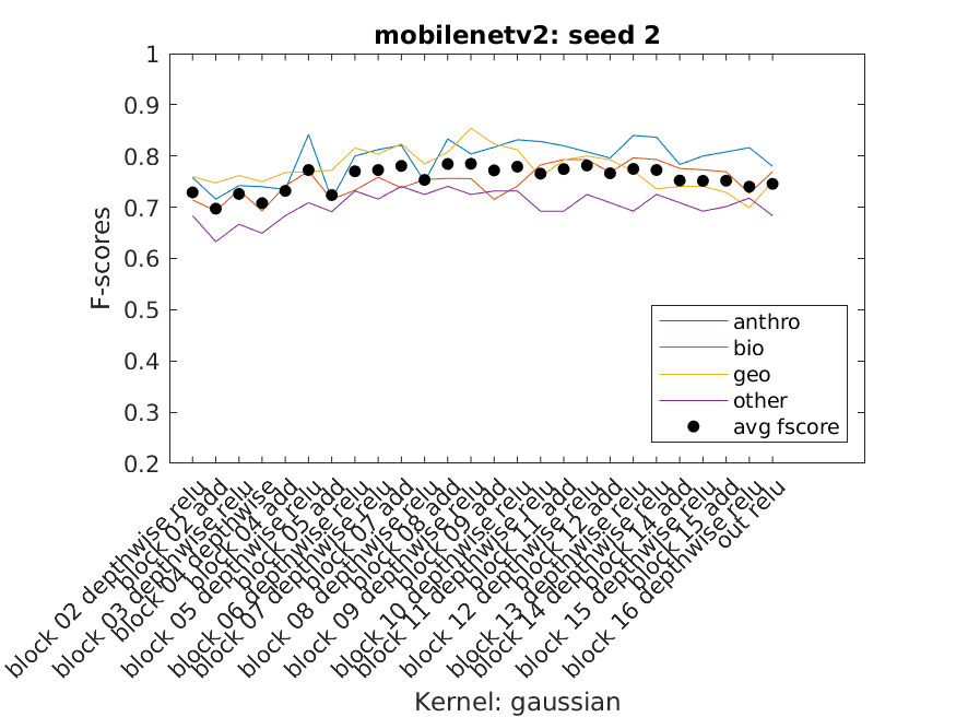
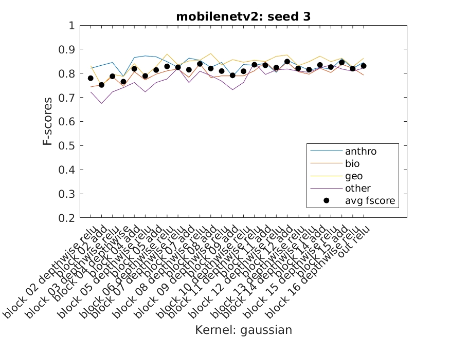
When just getting started most of the SVM usage was playing around to get an understanding of the data we had and how it performed with some generic SVM templates. Eventually three SVM templates were chosen to perform the bulk of the work. We used Bayesian Optimization as well as some of our own exploration to select the hyperparameters. Using a script we were able to extract multiple layer's features from a single network and use them to classify our data using the three templates as well as three seeded random data splits. The accuracy, f-score, and average f-score were saved which allowed us to then create data visuals. From there we could inspect the visuals to find those combinations that performed best and use them for the next part of the project.
Charts of the f-scores of each of the four categories performance across mobilenetv2 on three data splits

for s = 1:size(seeds,2)

	data_name = "svm_data_"+network+"/datastore/"+network+"_DS_s"+num2str(seeds(s));
	[training_Set, validation_Set, testing_Set] = getOriginalDataSplits(dir,seeds(s),data_name);

%         % Uncomment for OVER SAMPLING training set
%         training_Set = OverSampleTrainingSet(training_Set);
%         % Re-save the datastore
%         save(data_name, 'training_Set','validation_Set','testing_Set');

	for l=1:size(layers,2)
		[acc svm] = getSvms(net,network,layers(l),seeds(s));

		if hgstAcc < max(acc)
			hgstAcc = max(acc);
			hgstSvm = svm(find(acc == max(acc)));
		end

		if lwstAcc > min(acc)
			lwstAcc = min(acc);
			lwstSvm = svm(find(acc == min(acc)));
		end

	end

end
The Last Step and Results
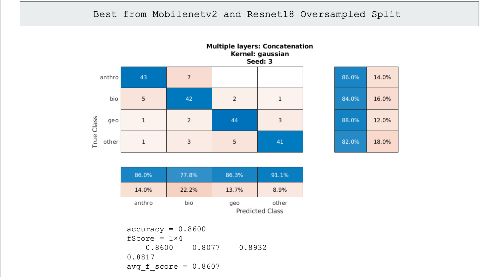
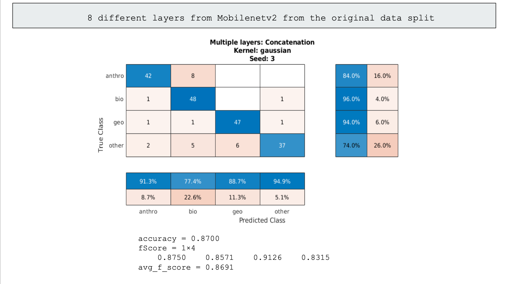
The last promising step of classification we used was ensemble learning. Generally in ensemble learning you would have multiple specialized classifiers that would work in tandum to identify an image, however none of our models were specialized and were all generalized in handling the data given. So instead we made due with using multiple high performing models, concatenated their classifications into an svm, and got a more roboust svm classifier that performed slightly better than the best models we had previously trained. This method however needs more time to be looked into, as with more fine-tuning of the models used in the data, we can take the models that handle each category the best and create a better model than the 86% and 87% we ultimately settled on.
86% Accuracy using the two best individual models
87% Accuracy using all of the best individual model's layers
Disscusion and Conclusion
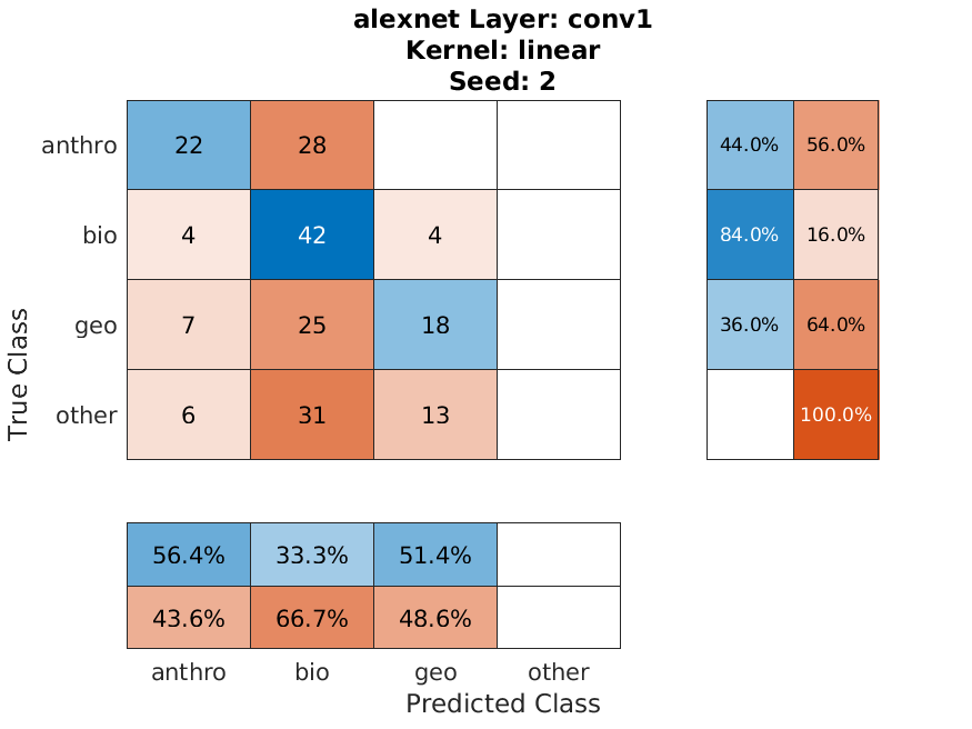
We were able to collect a lot of data about the performace of SVM's on Alexnet and Mobilenetv2. Shallow layers overall did worse than than the deeper layers with more robust features. Taking a look at the features can also provide clues as we move forward with feature extraction. To the right are the deep layer features of Alexnet and Mobilenetv2. It is interesting to note that the more complex and less distinct features of Mobilenetv2 perform better. Whereas the more detailed features of Alexnet seem not to complement the uniqueness of our data.

Mobilenetv2
Alexnet
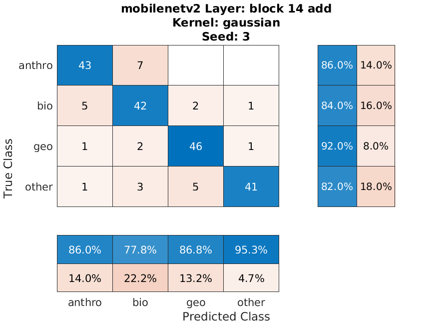
We were able to get reasonably good results considering the imbalance of our data. Below is the confusion chart of our best individual performing classification by "block_14_add" of Mobilenetv2 of the oversampled data split, and our worst performing classification by "Conv_1" of Alexnet of the original data split. The accuracies are 86% and 41% respectively.
Areas for Improvement
For what can be improved, we have a lot of ideas.
For ensemble learning, if we could implement the XenoCanto trained model in a python implementation of the code, we would most certainly have the best classifier in regards to identifying biophony (our worst performing category).
The removal of unecessary validation sets that could be added to the training sets as well as increasing the number of epochs would improve our accuracy.
We had to train many models, generally with 4 to 6 epochs each, so the inclusion of many more cycles could help the result. We must avoid overfitting by noticing when the testing accuracy starts to worsen.
Lastly, there were many other models that we hadn't had the chance to test on and many other layers that would've been nice to see how they perform.