Tree Classification David Holstedt, Nina Potts, Sean Callahan, Tairyn Addison

CS479: Classifying tree species using 3D point clouds of forest data

Introduction

The primary objective for our project was to utilize machine learning algorithms to detect forest tree species. In our approach, we looked at two CNN designs for analyzing the tree species: a voxel-based network and vector-based network. Our results will provide biologists with detailed information about the types of aboveground biomass (AGB) present in our forests.

Data

Our data was provided on behalf of Lisa Bentley, Ph.D. of the Sonoma State Biology department and Matthew Clark, Ph.D. of the SSU Geography, Environment, and Planning department. Bentley and her team, including graduate student, Breianne Forbes, collected 3-dimensional laser images of the forest. These terrestrial laser scanners save their data as a set of points represented in 3-dimensional space. The point datasets, or point clouds, typically include hundreds of thousands—even millions—of points for a single tree.

Computer science student, Alexander Barajas-Richie, ran the available laser point clouds through the Python script, TLSeperation. This script separates a single tree into wood only and leaf only point clouds.

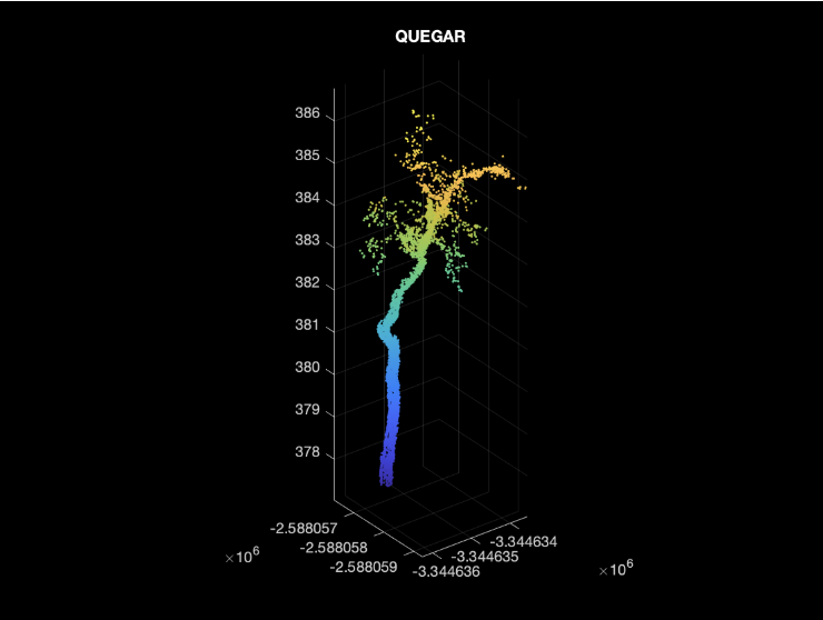
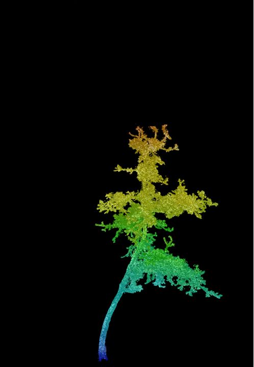
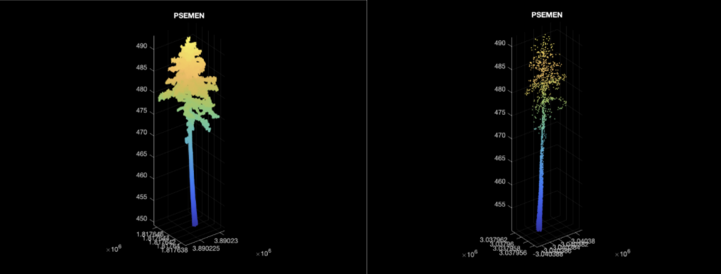
The figure below shows trees before cleaning, after outliers were removed, and a seperated wood only tree:

Each resulting tree data filename included the plot, quad, and tree number. For example,

c1_tls_p1342_tree1996_201026.wood.txt

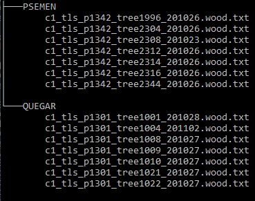
which follows the format: campaign_tls_plot#_tree#_date.(wood|leaves).txt

In order to train our network to utilize the tree species as a label, we needed a way to identify the tree species using only its filename. First, we wrote a MATLAB script to look up a tree in an Excel metadata file containing all the trees and their species. This posed a challenge when manually splitting our training and test sets. The MATLAB script would need to run to identify the species rather than managing it offline.

Thus, we wrote a program mktreedir that walks through a given unsorted data directory and matches trees to their species. Then the file is copied to a subdirectory named its respective species.

Using the wood only data we had only 3 unique species.

• (27) QUEGAR — Oregon oak (Quercus garryana)
• (10) PSEMEN — Douglas-fir (Pseudotsuga menziesii)
• (1) QUEAGR — Coast live oak (Quercus agrifolia)

Approach

Inevitably, we chose two approaches for classifing our trees. The first method we chose to explore was the vector based approach mentioned in the article “Effective machine and deep learning algorithms for wood filtering and tree species classification from terrestrial laser scanning”. Since PointNet++ was unavailable for MATLAB we had to use PointNet which we later found out was not a built in network. Our dataset was imbalanced and biased towards the QUEGAR species so we had to oversample the PSEMEN species so the network is not biased in choosing one over the other.

Different approaches as explained in the article. We focused on the approaches surrounded in red.

VoxNet

For the voxel based approach, we transformed the point cloud dataset by performing a random rotation about the z-axis, and applied a jitter to each point in the point cloud. This jitter adds a small amount of random variation to each point, and this is helpful in a smaller dataset to avoid overplotting. All of the point clouds were downsampled to 5,000 points using MATLAB’s pcdownsample built-in function. This considerably improved the speed of training for our point-based neural networks. By reducing the time to spatially bin the points, downsampling effectively reduced the training time of the voxelized approach as well. These images show the data before and after downsampling them.

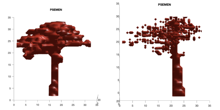
Point clouds before and after downsampling (top). Voxelized point clouds using 32x32x32 voxels (bottom).

After voxelization, we implemented transfer learning using a network trained on the Sydney Urban Objects dataset to replace the last learnable layer in VoxNet to be able to classify the trees based on our own classes.

We chose to use stochastic gradient descent with momentum for one of our training options. We found that when this was added it helped our training and testing sets to converge. Before doing this the gap between the training accuracy and validation accuracy was larger.

VoxNet Results

We also found that the uneven number of files for each tree species caused there to be a bias in the training data and overfit the validation data (shown in figure below on left). In an effort to fix this we oversampled the files to create an even number of each. We also decreased the batch size, increased the number of epochs, and increased the number of iterations per epoch.

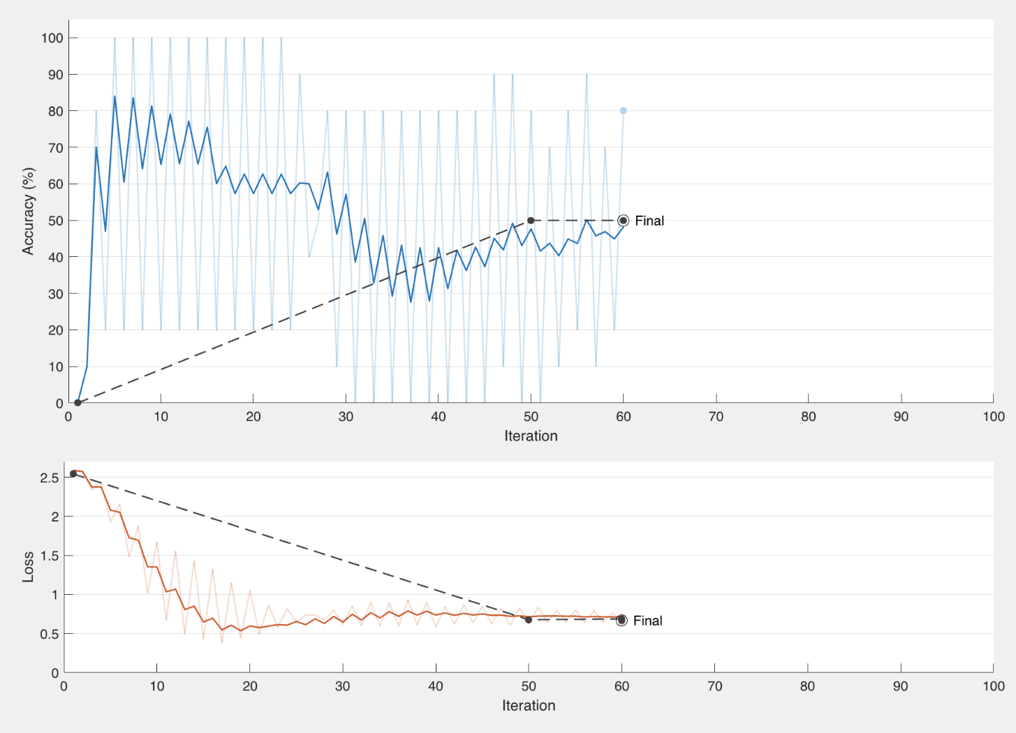
Two examples of training using data split in favor of QUEGAR.

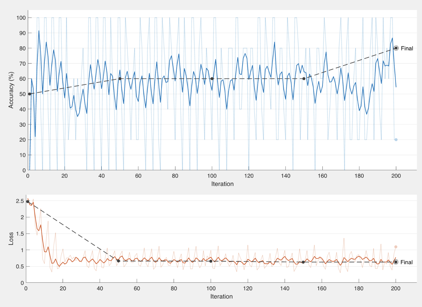
We then decided to try “leave one out cross-validation” so we could get a better idea of how our algorithm performs. For every trial we left one file out to put in our testing set, and we made sure not to include that file in our training data so there was not a bias. We did this for every file to cross-validate the performance and get a better understanding of each tree and how they are categorized. Here are some examples of our test runs:

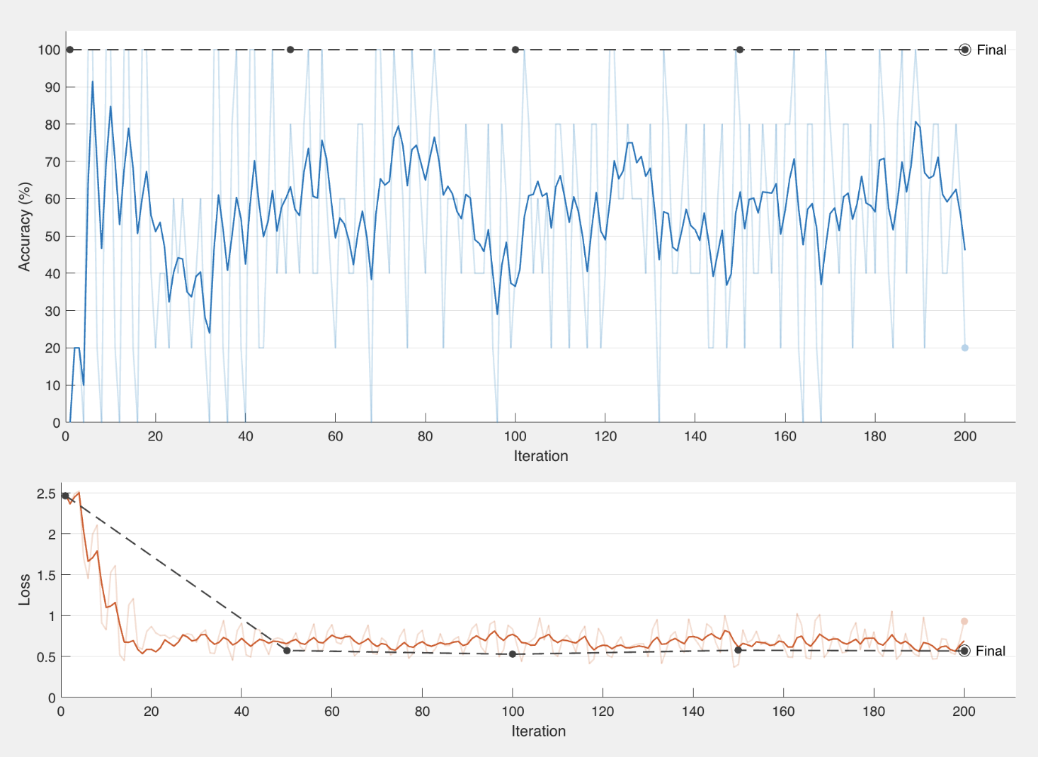
Examples of training results using leave one out cross-validation.

By doing these test runs we were able to figure out which files were harder to identify based off of their wood structures and duplicate those files to add in our training data. This gave us a more diversified and balanced training set for us to be able to classify trees because the structures that were previously hard to identify became more prevalent in our models.

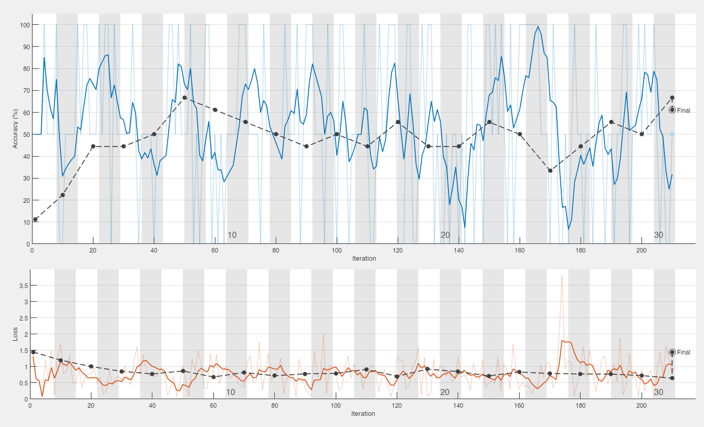
With continued training and the accuracy ranged from around 50-70% with our highest accuracy being 80% with an f-score of .7619. Highest results are shown in the figure below.

Graph of best results using VoxNet with 80% accuracy (left). Confusion matrix of that run (right).

PointNet

Another method we tried was the vector based approach, PointNet. Since PointNet++ (as discussed in this article) was unavailable for MATLAB, we had to use the original PointNet—which we later discovered to not have a built in CNN framework. To augment the point clouds, we downsampled them by 30 percent and jittered the points with Gaussian noise to create a random displacement field. Once we started training we realized that there was not any transfer learning happening. Without transfer learning, the results training using our dataset were abysmal. We began to explore other networks.

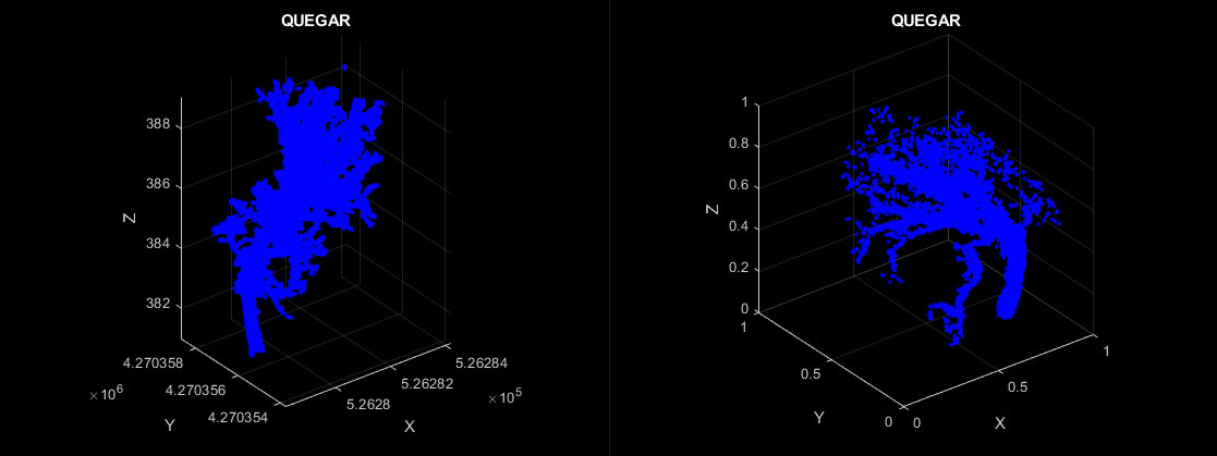
A tree (left) before augmentations. Same tree (right) showing various augmentations applied for PointNet.

3DmFVNet

To replace PointNet in our vector based approach, we selected 3DmFVNet as our new focus. 3DmFVNet uses Fisher Vectors to represent point clouds. Since inputs to CNN must be consistent, we downsampled the point clouds to a fixed number of points--in our case 1024 points. Furthermore, we performed similar augmentations to our previous approaches: random Z-axis rotations and jitter using Gaussian noise.

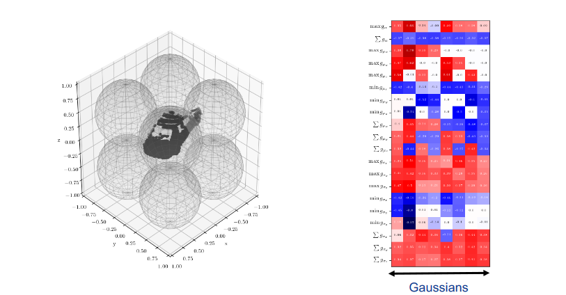
Example of how 3DmFVNet represents point clouds using a Gaussian Mixture Model (GMM)

Our 3DmFVNet MATLAB implementation comes from GitHub. In their tests, they downsampled all their point clouds to 4096 points. Due to GPU memory constraints, we had to downsample even further to 1024 points per tree. This noticeably reduced the granularity and feature distinction of the tree, but due to our limited resources this was a necessity. Further tests could be conducted with more appropriate hardware resources which should result in better accuracy given our limited data.

3DmFVNet Results

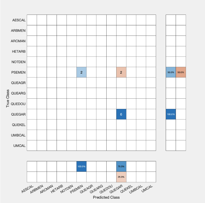
Our tests were conducted with 7 trees for each species in our training set and the rest in testing to avoid bias in the training set. Additionally, we conducted tests using the leave-one-out approach with 9 trees of each species in training and 1 tree in testing. This resulted in very similar results to the aforementioned dataset split. The following figure shows the best result conducted using 3DmFVNet on the data provided.

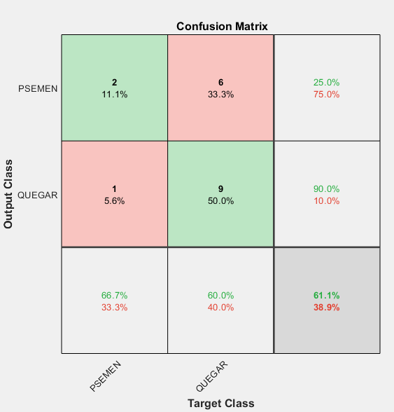
3DmFVNet graph and confusion matrix with accuracy of 61%.

Our results showed a slight improvement over a trivial 50/50 guess between our two species. With QUEGAR mostly being classified correctly. Most of our testing resulted in an accuracy of 55-60% and an f-score of 0.36.

Conclusion