CS 479 : Animal Detection with Active Learning
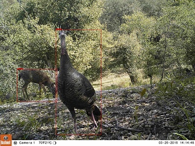
Detection of a deer and a turkey.
The focus of our project was animal detection for the purpose of tracking biodiversity via images captured by camera traps in a nature reserve. Our dataset comes from the Fairfield Osbourne Preserve here in Sonoma County, California and consists of roughly 25,000 labeled images of the wildlife that lives there. The core problem we were trying to solve was the efficiency of animal labeling in machine learning. Manually labeling images is extremely slow and takes away from the limited resources that ecologists have. While standard machine learning methods have greatly improved this process, they require a large pre-existing training set that must be well labeled. To combat this limitation and further improve machine learning in image labeling, we implemented the Active Learning algorithm which requires fewer labels and can ideally improve accuracy. The essential milestones of our project are as follows:
- Run dataset through object detection script and crop out areas of interest.
- Group images by isolated camera events to prevent bias.
- Implement oversampling to make up for imbalanced animal categories.
- Train machine learning model on improved dataset.
- Implement k-Fold and Leave-One-Camera-Out cross-validation to estimate accuracy.
- Build and utilize Active Learning algorithm with trained model.
Applying Active Learning to our classification model provided us with mixed results. Our Active Learning network peaked around 76% accuracy and f_scores remained low. However, this was in part due to the quality of our dataset. The number of images for each animal varied greatly, with the number of images containing no animals being more than twice the size of the next largest category, deer. There were also numerous mislabeled images, which mistrained the classifier and made analyzing results more difficult.
Building the Classification Model
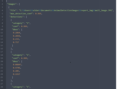
The first major goal in our project was building a machine learning model that could classify different types of animals. The initial step involved in this was running our dataset through the CameraTrap animal detection script built by Microsoft AI for Earth which can be found here. This Python script provided us with a JSON file that contained the coordinates of each animal it detected in each image we gave it. We then used MatLab to parse that file and crop down the images to feature the animals as clearly as possible. A visual representation of what the detector does is shown below, alongside what its equivalent JSON output looks like. (Full JSON file can be found here)
The next step involved grouping together specific images. The camera traps that created our dataset are set up in such a way that, when they detect movement, they take a burst of three pictures. Together, these three images are a single event. In order to prevent bias in our classification network, we needed to make sure that each event had all three of its images in either the training set or the test set. We wrote a Python script to group the images by event and prevent bias from occurring in this way.
The third step in improving our dataset was oversampling. This process involves duplicating the images in the categories with fewer images until they equal the number of images in the largest category. Due to the extreme imbalance in the categories of our dataset, this resulted in some images being duplicated thousands of times. For example, there were only five pictures of hawks in our dataset, compared with 4,272 deer pictures. The oversampling technique we used in MatLab would duplicate those five hawk images over and over again. While this did help our results somewhat, oversampling seems to be more effective when the imbalance of categories is less extreme.
Once we had refined and improved our dataset as much as possible, we used it to train a classification model and implemented k-Fold and Leave-One-Camera-Out cross-validation to estimate the accuracy of our model. In k-Fold cross-validation, the testing data is randomly split into k groups. It trains the model on k-1 of the groups and tests the model on the remaining group. Leave-One-Camera-Out cross-validation is virtually the same process but differs in the way the data is split up. In this method, the dataset is organized by which images were captured by a specific camera. Following the k-Fold logic, it then trains the model on all cameras' images except for one, and tests it on that last camera's images.
The Active Learning Algorithm
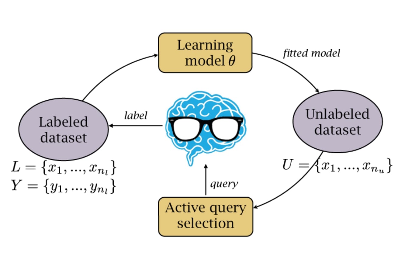
An active learning model allows us to label unlabeled images efficiently and accurately. The main benefits of using such a model is that you can improve a current network using unlabeled images without needing to manually label every image. Without an active learning model, machine learning programmers would be required to label every training and testing image by hand. Of course, you might ask, why not just manually label some of the data without building an active learning model to save some time? Another benefit of using an active learning model is that you can use it to determine which data is useful for training your classifier, and focus the human's effort into accurately labeling this data. This means the "beneficial but hard to classify" images are classified by the human while the easy to classify images are classified by the network. For our purposes, images are considered useful if they have features not present much in the training data. As such, an active learning model can train a network better than if using a random approach, and each iteration should return slightly better results for the next iteration.
The specific active learning algorithm we built operates as follows:
%psuedocode
for i = 1:num_training_images{
	-Classify single training image
	-Find top two most confident class predictions
	-Find differnence between second_most_confident and most_confident

	%Query strategy
	if (difference < threshold){
		-Manually label training image
	}
	else{
		-Auto label training image
	}

	-Add labeled image to training set
	if(training set big enough) == 0){
		-Train network on training set
		-Clear training set
		-Classify test set and print accuracy
	}
}
The query strategy is what you use to determine which images should be labeled by hand and which should be labeled automatically. Originally, we checked only the most confident class of each image, but this is not a good method. Simply taking the most confident class totally disregards the other classes, and since the data is there we should take advantage of it. Instead of a least confidence based strategy, we implemented a margin strategy. This involves retrieving the top two most confident classes, subtracting one from the other, and finding the difference. Low differences imply the network is having trouble splitting the difference between classes, and thus should be manually looked at. The main idea here is that ignoring the other classs' confidence levels is a waste of valuable information that could otherwise help a better decision be made. Once enough images are added to the training set, we test the network by finding the percentage of correct classifications on the testing data.
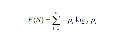
As a result of the active learning algorithm, were able to achieve a positive trend of correctly classified testing images after several iterations, as well as label unlabeled data much quicker than if we had done so manually. While the approach was overall successful, there are some drawbacks that need to be considered. Firstly, this approach does not take bias into account when evaluating the performance on the testing data. This is problematic because a single event can have multiple images that are similar, and cross validation is necessary to solve this problem. Secondly, margin sampling is still not the best query strategy. While margin sampling takes more variables into account than least confidence sampling, using all classs' confidence results is still a better method. This can be done using entropy sampling, which uses a formula (shown above) that requires the confidence result from all classes.
Results
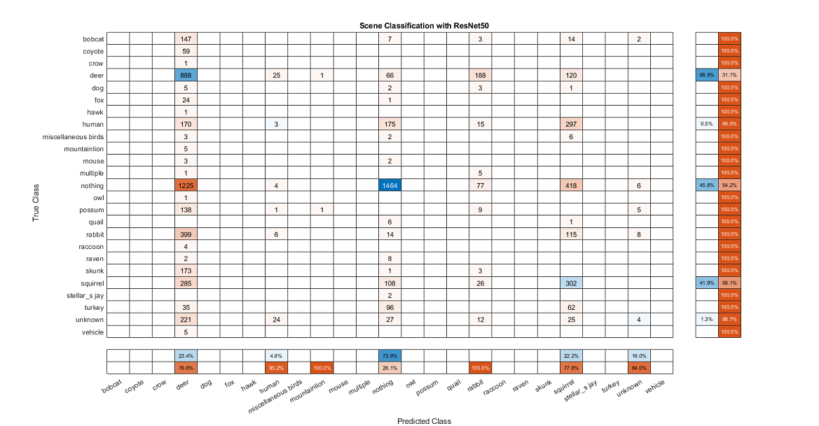
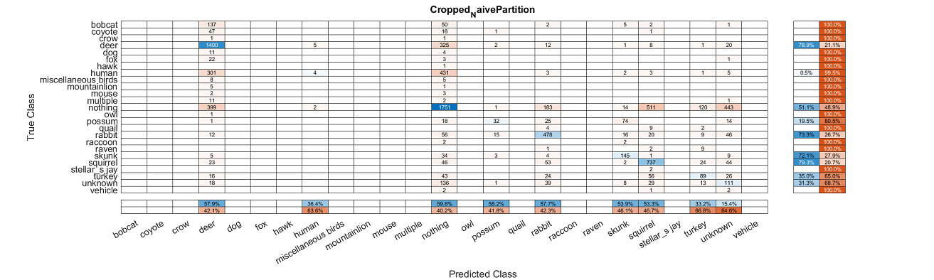
The images of confusion matrices below track the evolution and improvement of our classification model as we refined our dataset and added features.
Training and testing the base dataset with a naive partition provided very poor results with an average fscore of 0.2475.
After running the dataset through the object detection script and cropping them down, there was some improvement, but still rather poor accuracy with an average fscore of 0.441 and 53.42% accuracy.
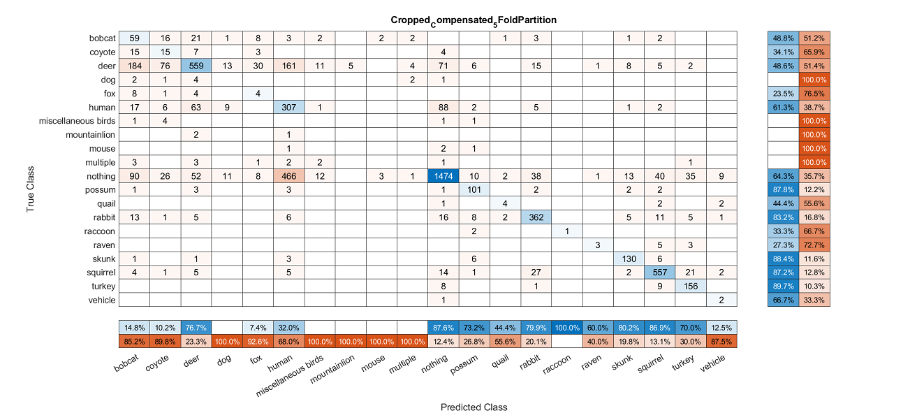
In this test, we removed the nothing category of images as well as a few other categories that had very few images. To test accuracy, we implemented k-Fold cross-validation with a k value of 5, but used only one of the folds for training. This gave us an average fscore of .435 and our highest accuracy at 71.88%.
Conclusions
While we weren't thrilled with the accuracy of our end product, we were still able to build a reasonably accurate animal classification model that incorporates Active Learning. Our most significant challenge was overcoming the flaws in our dataset. The vast disparity in number and quality of images for each category along with mislabeling created a lot of issues in training our model that we were only able to partially remedy. Provided more time, we would have liked to find a balanced and well-curated dataset that we could train our model with and compare the results to what we got with our dataset. That being said, one of the exciting things about this model is its portability. Due to the properties of the Active Learning algorithm, the model can be quickly and easily deployed to new environments with minimal training data required. For example, the model could easily be trained on animal images from an African nature preserve that has much different animals from the ones at the Fairfield Osbourne Preserve in Sonoma County. It is a tool that could be used by ecologists to save time and energy and devote those precious resources elsewhere.