Covid19 Detection
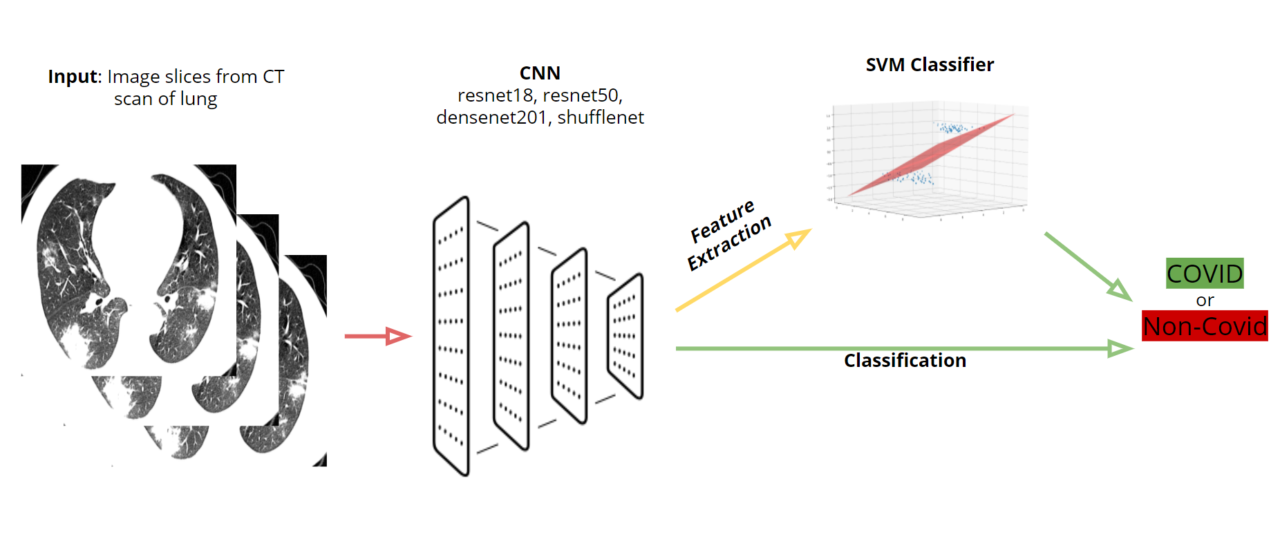
Our team's goal was to look into the existing research on COVID-19 detection through image recognition and create multiple models and explore different methods for classification using CT scan data as our input.
Our datasets were as follows:
The first preliminary testing we did was attempting to reproduce Dr. Pham's results he obtained from using a random data split with 80% of the images going to training and 20% to testing. The CNNs we tested were resnet18, resnet50, densenet201, and shufflenet. For each CNN, we tested this data split one time without data augmentation (rotations, reflections, translations, and scaling) and another time with data augmentations on the images. For each test, the mean accuracy, mean F-score, and their standard deviations were calculated.
Similarly to Dr. Pham, we found that not using any data augmentations with a random data split led to higher accuracies and F-scores for the four specific CNNs that we tested. The accuracies achieved were almost 95% for each network. This gave suspicions that the accuracies were a bit too high so we investigated a technique called leave-one-patient-out cross validation to remove bias and get accuracies that are more represntative of how well the CNNs performed with our dataset.
Leave-one-patient-out cross validation is a process where the entire dataset is divided so that each patient’s images are only grouped with their own lung images and put into an individual subset. In our case, we have 384 patients so we would have 384 subsets. Each subset represents one iteration where we will end up training and testing our network. For each iteration, one subset will be used for testing and the rest will be part of training. For the preliminary testing, after training the network each iteration, the accuracy and F-score was calculated. After every subset was tested, we calculate the average mean and F-score along with their standard deviations. This cross-validation is useful because it allows us to test our networks with the same dataset multiple times. This method also ensures that a patient’s images won’t be in training and testing at the same time, effectively getting rid of any bias that could occur if we had a random data split.
For leave-one-out, the first thing we do is create a folder called leave_out that contains training and testing folders for noncovid and covid images. At first, all images will go into the training folder. Depending on which patient number we are looking at, we will move that patient's images from the training folder into the testing folder then train our network as usual.
% Go through the COVID images and get the images that need to be moved.
if(isCOVID == 1)
	for i = 1:covid_size
		if(strcmp(COVID_sheet.Var2{i},patient_id) == 1)
			images_to_move = [images_to_move ; COVID_sheet.Var1{i}];
		end
	end
end

% Go through the nonCOVID images and get the images that need to be moved.
if(isCOVID == 0)
	for i = 1:noncovid_size
		if(strcmp(nonCOVID_sheet.Var3{i},patient_id) == 1)
			images_to_move = [images_to_move ; nonCOVID_sheet.Var2{i}];
		end
	end
end

% Get number of images to move.
move_num = size(images_to_move,1);

% Move the COVID patient's images into the validation folder.
if(isCOVID == 1)
	for i = 1:move_num
		file_name = images_to_move(i);
		movefile(fullfile(train_covid_path, file_name + "*"), val_covid_path);
	end
end

% Move the nonCOVID patient's images into the validation folder.
if(isCOVID == 0)
	for i = 1:move_num
		file_name = images_to_move(i);
		movefile(fullfile(train_noncovid_path, file_name + "*"), val_noncovid_path);
	end
end
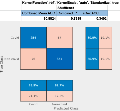
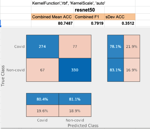
For the preliminary testing of transfer learning with leave-one-out validation, we found that resnet50 had the highest accuracy and F-score while shufflenet had the lowest accuracy and F-score. Each network obtained an accuracy of at least 75%. The results obtained from using leave-one-out cross validation is significantly lower and have a large range of standard deviations compared to the results obtained with random data splits. This is because randomly spliting the data leads the bias which increases the accuracy and F-score obtained by the CNN.
For the preliminary testing of transfer learning with leave-one-out validation, we found that resnet50 had the highest accuracy and F-score while shufflenet had the lowest accuracy and F-score. Each network obtained an accuracy of at least 75%.
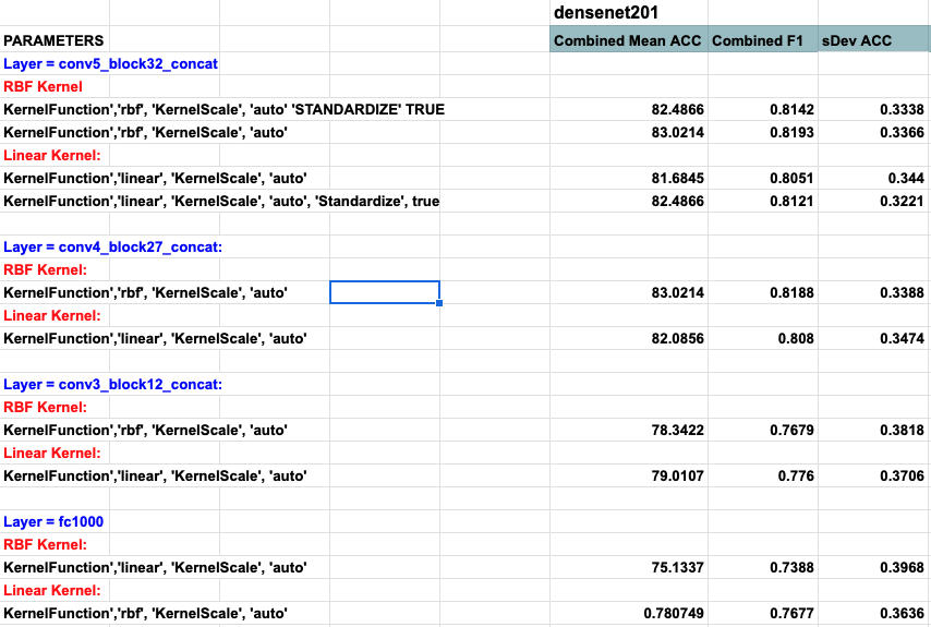
Densenet201 performed the best across the board for the SVM classifier. Shufflenet was close behind, Resnet50 following that. Resnet18 performed the worse. This was interesting to see because resnet18 performed the best for
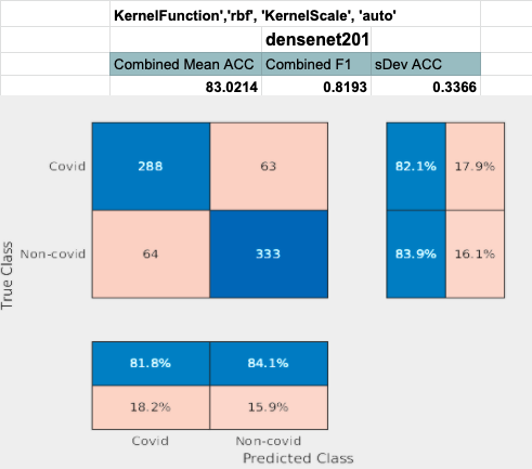
Densenet performed the best with feature extraction. The last concatination layer was used for this test. (conv5_block32_concat)
Shufflenet performed the 2nd best. Layer node_198 was used to achieve this result.

Restnet50 performed 3rd best. Layer add_16 was used to achieve this result.

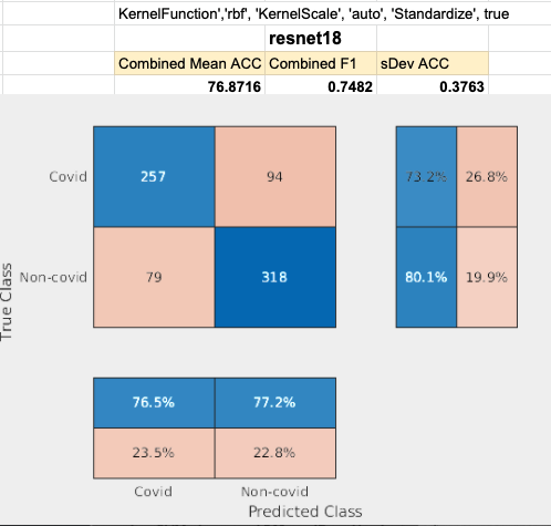
Restnet18 performed by far the worst. Layer pool5 was used to achieve this result.

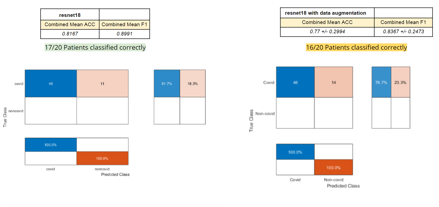
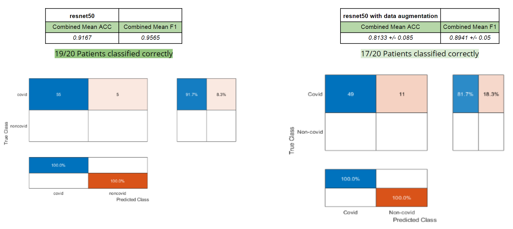
For our final testing, we used the same four CNNs (resnet18, resnet50, densenet201, and shufflenet). The entire UCSD dataset was put into training and the three image slices for each patient (from CT scans from Coronacase and Radiopaedia) was put into our testing set. We tested with transfer learning with and without data augmentation, this time without doing leave-one-out cross validation. When there were data augmentations, we trained and tested the network five times and calculated the standard deviation and average accuracy and F-score. We also tested this dataset with feature extraction with a SVM classifier and calculated the accuracy and F-score. To determine if a patient should be labelled as having COVID, two or more of the three images had to be classified as containing COVID.
Both methods for resnet18 yielded similar results (Figure 2) with a 81.67% accuracy without data augmentation and 77% accuracy without data augmentation.
Resnet50 performed much better without data augmentations, getting around a 10% higher accuracy than with data augmentation (Figure 3).
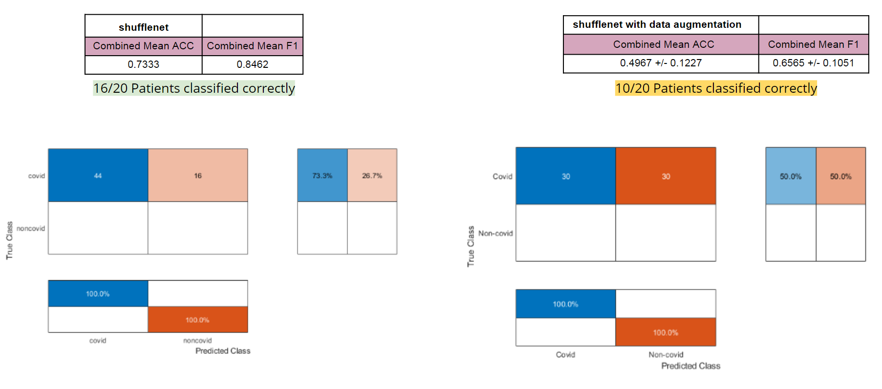
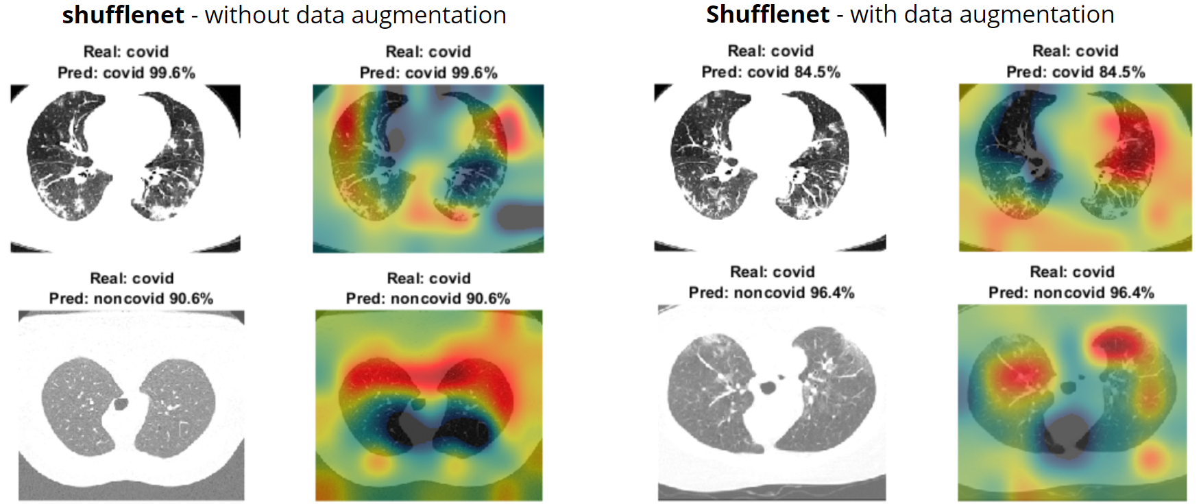
Shufflenet performed significantly worse when training with data augmentation, getting the worse accuracy out of all of the other networks (Figure 4). Using this method, shufflenet was only able to identify half of the patients as having COVID.
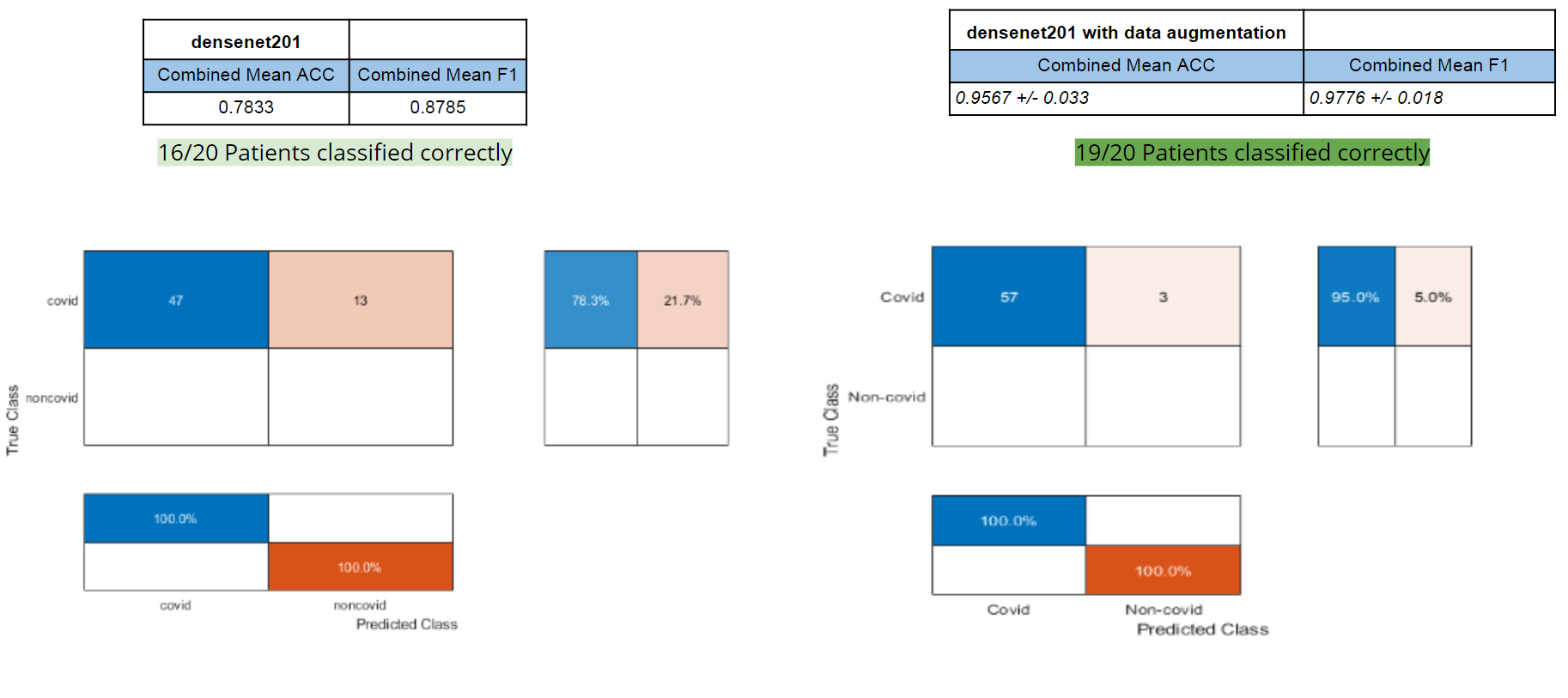
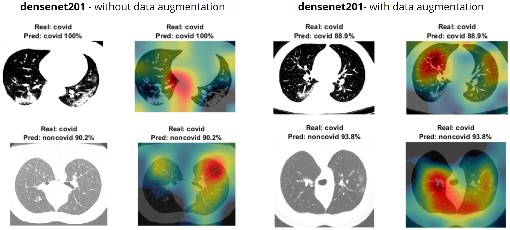
Densenet201 was the only network that performed better with data augmentation as shown by Figure 5. For our final tests with transfer learning, this network got the best accuracy and FScore whiel maintaining a very low standard deviation for both. Densenet201 was able to correctly identify that 190 out of the 20 patients had COVID.

Since most Neural Networks are looked at as black boxes, naturally our group was curious as to what was going on inside and what our CNN's were basing their decision making process on. Thankfully we were introduced to the option of using Heat-Mapping techniques that could show us what image features were being considered more heavily by each of our CNN's. The heat mapping method we chose was "Class Activation Mapping". To do Class Activation Mapping, we needed to use the final Convolutional layer of our CNN as input. This layer holds matrices that represent the feature-maps. We first get the max scores for each feature map through a process called Global Average Pooling. To do Global Average Pooling we must take the average of each feature map by summing all the values and dividing by the number of elements. This gives us K scores for K features maps. We can then get a score for a given class by multiply each of the weights that connect from this Global Average Pooling number to that class by the Global Average Pooling number and summing up those results (This sometime already happens in the form of a "fully connected layer" that follows the last Convolutional layer, as can be seen in densenet201 for example).
imageActivations = activations(net,imResized,layerName);
scores = squeeze(mean(imageActivations,[1 2]));
fcWeights = net.Layers(end-2).Weights;
fcBias = net.Layers(end-2).Bias;
scores =  fcWeights*scores + fcBias;
After we have that score we can now obtain the Heat Map by multiplying each of the weights directly with its respective feature map and summing them up.
[~,classIds] = maxk(scores,2);
weightVector = shiftdim(fcWeights(classIds(1),:),-1);
classActivationMap = sum(imageActivations.*weightVector,3);
We then use a nice function provided on a mathworks documentation article to help us properly display the heatmap.
subplot(1,2,2)
CAMshow(im,classActivationMap)
title(string(labels) + ", " + string(maxScores));
function CAMshow(im,CAM)
imSize = size(im);
CAM = imresize(CAM,imSize(1:2));
CAM = normalizeImage(CAM);
CAM(CAM < 0.2) = 0;
cmap = jet(255).*linspace(0,1,255);
CAM = ind2rgb(uint8(CAM*255),cmap)*255;
combinedImage = double(rgb2gray(im))/2 + CAM;
combinedImage = normalizeImage(combinedImage)*255;
imshow(uint8(combinedImage));
end
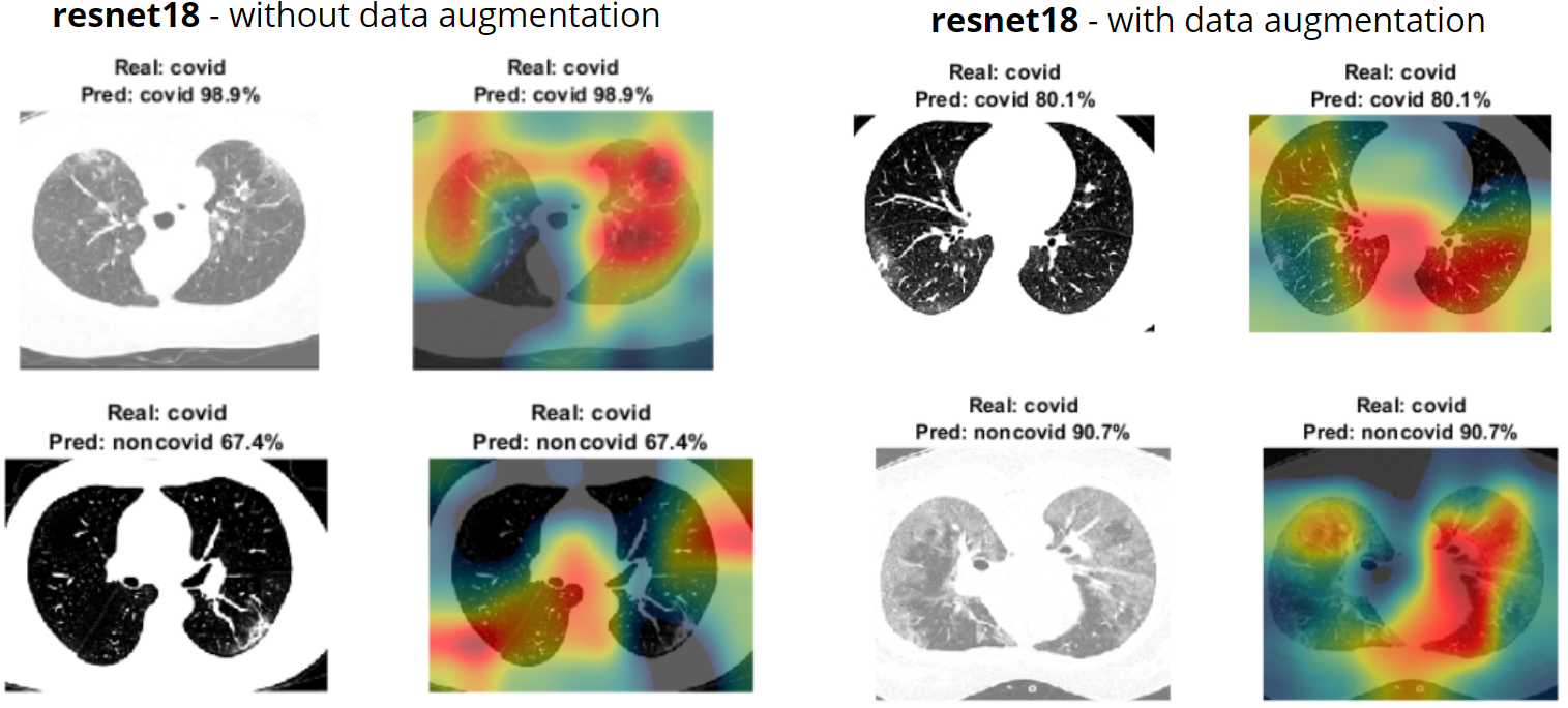
The heatmaps for resnet18 with data augmentation had differing results than heatmaps without data augmentations as seen by Figure 7. When there was data augmentation, the heatmap showed that the CNN was looking between the lungs rather than inside of them for classification.
Resnet50 performed better than resnet18 as seen in Figure 8. With non-augmented data, the data classification heavily ultilized the areas outside the actual lungs. With the augmented data, we can see that there was a large focus inside of the patient's lungs.

Shufflenet did very poorly as displayed by Figure 9. Without data augmentation, the inside of the lungs weren't being looked at very often and with data augmentations, it was only looking inside the lungs sometimes, but would include portions of the outside as well.
Densenet201 performed the best with augmented data. With data augmentation, the CNN consistently looks inside the lungs to classify the images (Figure 10). With non-augmented data, the model would look both inside and outside of the lungs.
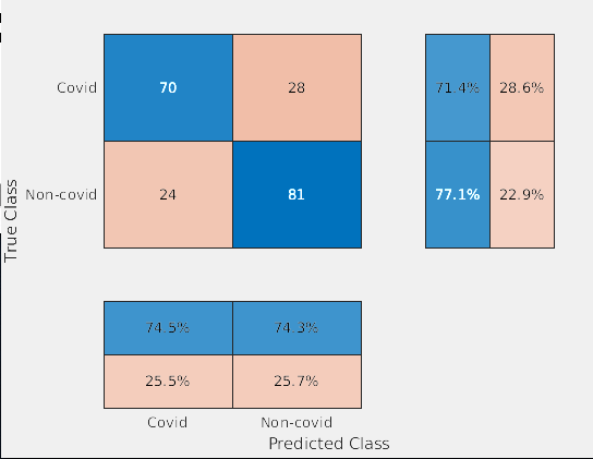
For our final data set, The entire UCSD dataset was put into training and the three image slices for each patient (from CT scans from Coronacase and Radiopaedia) were put into our testing set. This allowed us to train upon a large amount of data. The one problem with our final data set is the fact we have no NON-covid images for our testing set. This is why the bottom of the confusion matrix is blank (due to there being no false positive and no true negatives). In future tests we would like to integrate NON-covid images into our testing set.

Using our best parameters from what we learned with Leave One Out SVM, we achieved high accuracies for both Resnet18 and Resnet50.
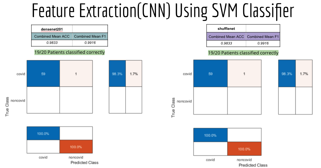
Once again using our best parameters from what we learned with Leave One Out SVM, we achieved high accuracies for both Densenet201 and Shufflenet.
Strangely 3 of our networks (Densenet201, Shufflenet, and Resnet18) performed the same. All 3 classified 19/20 covid patients successfully. In the future., we can explore why this is happening and see if its consistent. The inclusion of NON-covid patients in the testing set could possibly help these strange results.
bag = bagOfFeatures(imdsTrain);
optionsSVM = templateSVM('KernelFunction', 'rbf', 'KernelScale', 'auto', 'Standardize', true)
categoryClassifier = trainImageCategoryClassifier(imdsTrain, bag,'LearnerOptions', optionsSVM);

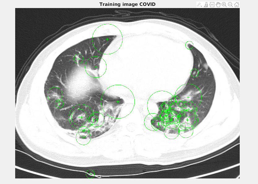
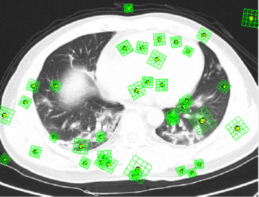
SURF was fascinating to visualize. Using an rbf kernel we were able to produce our FScore and Accuracy. In the future we would like to look further into the possibilities of SURF, perhaps tuning parameters. We achieved 75.37% accuracy and a FScore of .7135
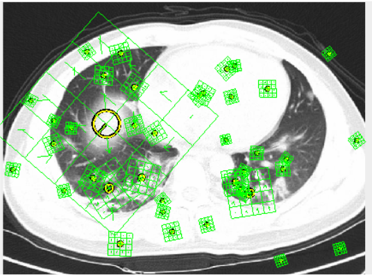
SIFT seemed to pick up features out of the lung region. This was not what we wanted. However, with more tuning it could be used to produce better results in the future.
We have yet to collect data with SIFT. Despite the lack of data it was interesting to see the difference in feature extraction.
Although we have done extensive testing, our models are not actually detecting whether an image of a lung has COVID-19. What they are finding is whether or not these lungs have features of viral pneumonia. The reason why we are able to say that the specific type of viral pneumonia is found is because we are in a middle of a pandemic. This means that this is is not the best clinical way to find if someone has COVID-19 or not. Although we are not experts with this type of data, it looked like some COVID CT images had no pneumonia features in a few UCSD Covid images and there were pneumonia features present in some UCSD non-Covid CT images.
Pham, T.D. A comprehensive study on classification of COVID-19 on computed tomography with pretrained convolutional neural networks. Sci Rep 10, 16942 (2020). https://doi.org/10.1038/s41598-020-74164-z