CS 479 :Classifying Sigma Clasts in Geological Formation
Introduction
To incentivize the participation and contribution to the growth of an earth-science-based cyberinfrastructure, analytical environments need to be developed that allow automatic analysis and classification of data from connected data repositories. The purpose of this study is to investigate a machine learning technique for automatically detecting shear-sense-indicating clasts (i.e., sigma or delta clasts and mica fish) in photomicrographs, and finding their shear sense (i.e., sinistral (CCW) or dextral (CW) shearing).
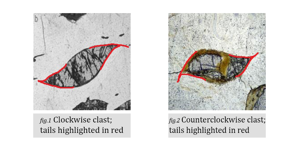
Figure 1 is an example of a CW clast and figure 2 of a CCW clast. Though subtle, the most important difference between each example are the tails. In previous experiments, our attempts at classification have turned poor results, typically reaching 40% – 70% accuracy and an F1-Score of ≤ 0.6 We suspect our previous results were poor due to the model used. Previously we used a transfer learning approach. We utilized various pretrained networks and connected a small custom network to fine tune the features extracted from the base CNN. However, our dataset size was not sufficient for this type of model. Thus, dataset augmentations, feature extraction, and classification methods were tested to explore how other models performed on this dataset. Feature extractors included CNNs, SIFT and classification models included CNNs (transfer learning), Bag of Words (SVM and Naïve Bayes), and GANs.
- Extract Features
- SIFT
- CNN
- Classify Features
- SVM
- GAN
- Generate/Augment Images
- Gan
- WGAN
- Augmentation
- Gan
Goals:
Dataset
By using these methods we were able to try multiple datasets. We only had 103 original images at first. This is not an appropriate sample size to be able to train a successful model. Using the methods of data augmentation and image genration through GAN, we were able to increase our dataset to over 800 images.
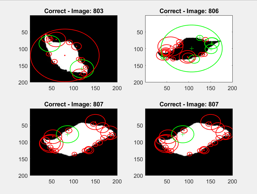
Our first issue with the data was the level of noise in each image.
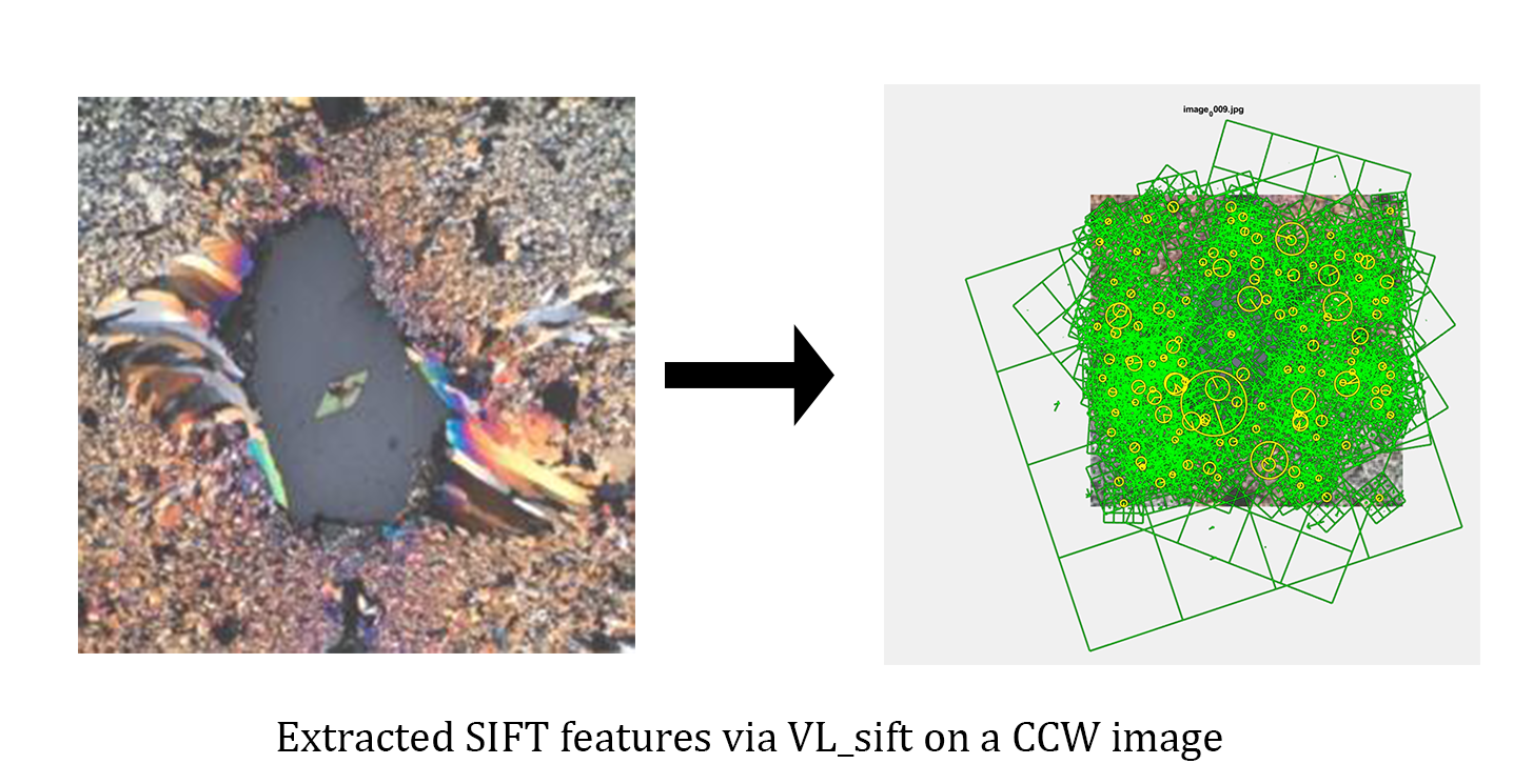
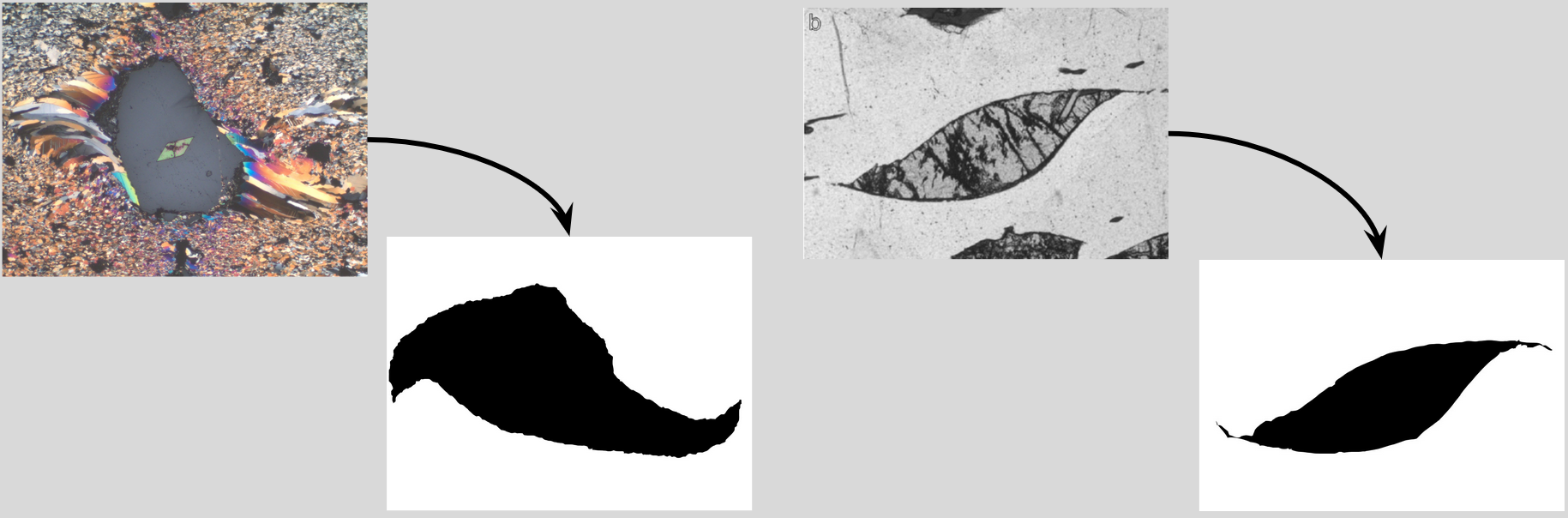
The above figure visualizes all features extracted from the image. Since we are only concerned about the central clast figure, we label any features outside of that shape as “noise”. Thus, to test CW/CCW classification in an ideal environment, we made “synthetic” images (below figure). These were hand drawn traces of the clast silhouette. The tails were exaggerated to make the orientation more pronounced.
Augmentations
Our original dataset comprised of 103 images, which is far from ideal. To compensate, we artificially added to the dataset by augmenting the images.
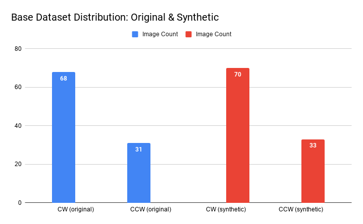
Augmentations included horizontal flip (converts a CW clast to CCW and vice versa), color inversion, and a combination of the two. We applied these augmentations to each original and each synthetic image. Our “combo” dataset included all original images with all augmentations, plus all synthetic images with all augmentations. This method not only increased the dataset size but addressed the issue of class imbalance.

Approaches and Algorithms
Each member took a slightly different approach with the dataset provided. We used a SIFT feature extractor with a BoW Classifier (Naive Bayes & SVM), CNN feature extractor with a SVM classifier, CNN feature extractor and classifier via Transfer Leraning and image generation and classification via a GAN and an augmentation script.
SIFT feature extraction with Bag of Words Classifier (SVM Model)
SIFT & VL_Sift
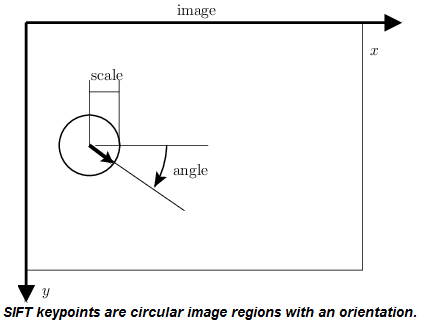
SIFT, or Scale-Invariant Feature Transform is a feature extraction algorithm. The primary advantage of SIFT features are their invariance to object variability. For example, SIFT features could still perform well even if the object in an image was rotated, shifted, put in low light, or transformed in some way. The VLFeat library was used to extract SIFT features.
VL_sift parameters
All default parameters were used, except for the edge threshold. EdgeThresh (function parameter name) affects the SIFT detector (the part of VL_sift that locates the features) by eliminating the peaks of the difference of gaussian space whose curvature is too small. Essentially, this makes the detector return features that are “tighter” to the objects of interest.

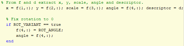

Normally, sift features are invariant to orientation. However, our classification problem detects orientation in clasts. By making sift features variant to rotation, the model performance may increase.

Features were made variant to rotation by manually adjusting the angle of all SIFT features to an angle of 0. ROT_ANGLE could be adjusted to fix the features to any specific orientation.
SVM
Support Vector Machines are a discriminative classification technique that, given an image, calculate the probability of a class. The probabilities are generated by the model space boundaries.
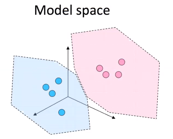
Essentially, when the SVM is trained, the model space groups clusters of categories and draws boundaries around the clusters. When a test image is input, the SVM calculates the probability of its class based on those boundaries and clusters (depending on the specified probability calculation).
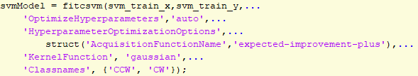
SVM Parameters
These are the parameters used for the built-in Matlab function fticsvm.
SIFT feature extraction with Bag of Words Classifier (Naive Bayes Model)
- SIFT with Bag of Words (BoW)
- Used the Navie Bayes model classifier to make predictions of different classes based on the various attributes
- Parameters Changed and Datasets Used:
%DATASET = 'og'; % DATASET = 'og_clrInv'; % DATASET = 'og_flip'; % DATASET = 'og_flip_clrInv'; % DATASET = 'syn'; % DATASET = 'syn_clrInv'; % DATASET = 'syn_flip' % DATASET = 'syn_flip_clrInv'; DATASET = 'og_syn_combined'; % use these sizes for 'og' %CCW_size = 31; %CW_size = 68; %use these sizes for 'combined' CCW_size = 404; CW_size = 404; % use these sizes for 'syn' sets % CCW_size = 33; % CW_size = 70; --VECTOR QUANTIZATION SETTINGS-- %% Number of entries in codebook VQ.Codebook_Size = 800; % Changed from 300 - Algorithm for Naive Bayes:
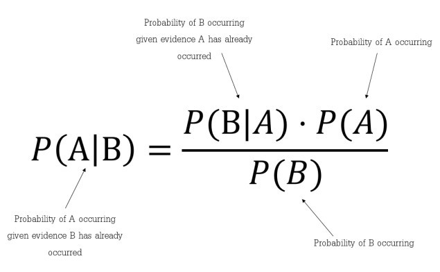
- Where B = class and A = data
CNN feature extractor with SVM classifer
- Used a Convolutional Neural Netowrk to extract features and use a Support Vector Machine to classify.
- Parameters:
options = statset('UseParallel',true); t = templateSVM('Standardize',true,'KernelFunction',"gaussian"); classifier = fitcecoc(featuresTrain,YTrain,'Learners',t, 'OptimizeHyperparameters', 'auto', 'OptimizeHyperparameters', ... "auto",'HyperparameterOptimizationOptions', struct('AcquisitionFunctionName', ... 'expected-improvement-plus'), 'HyperparameterOptimizationOptions',struct('MaxObjectiveEvaluations',100), 'Options' , options); - Algorithm:
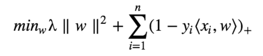
- Loss Function for SVM:
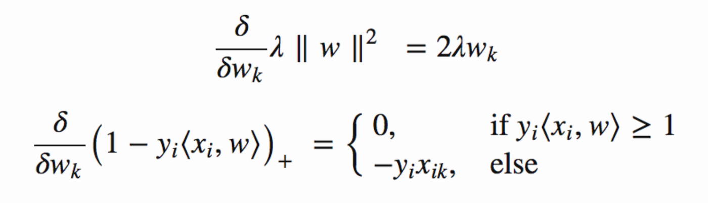
- Gradient Function:
CNN with Transfer Learning
- Used a pretrained CNN with an additional layer
- Algorithms for GoogLeNet are not available at this time
- Parameters:
miniBatchSize = 6;
valFrequency = floor(numel(augimdsTrain.Files)/miniBatchSize);
options = trainingOptions('sgdm', ...
'MiniBatchSize',miniBatchSize, ...
'MaxEpochs',50, ...
'InitialLearnRate',1e-3, ...
'Shuffle','every-epoch', ...
'ValidationData',augimdsValidation, ...
'ValidationFrequency',valFrequency, ...
'Verbose',false, ...
'Plots','training-progress', ...
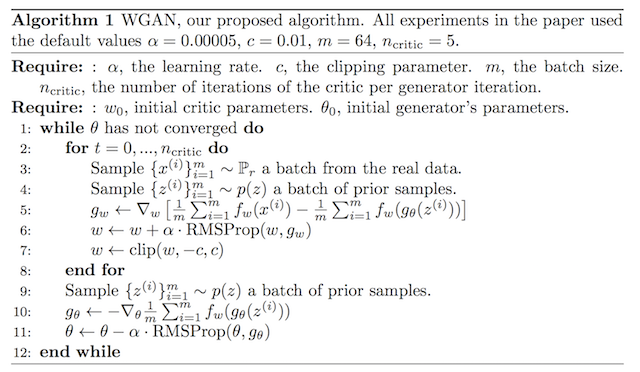
'ExecutionEnvironment','parallel');Wasserstein GAN
- Used to generate new images for expanding the dataset
- Parameters:
n_epochs = 800
z_dim = 64
display_step = 25
batch_size = 12
lr = 0.000075
beta_1 = 0.5
beta_2 = 0.999
c_lambda = 10
crit_repeats = 3
device = 'cpu'
New Methods Used
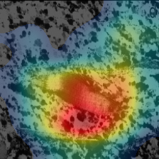
Using a heat map to verify feature dectection in the SVM classifier
for i = 1 : 647
    im = readimage(imdsTrain,idx(i));
    if(size(im, 3) == 1)
        im = ind2rgb(im, map);
    end
    im = imresize(im, [224 224]);
    imageActivations = activations(net,im,layer);
    scores = squeeze(mean(imageActivations,[1 2]));

    fcWeights = net.Layers(end-2).Weights;
    fcBias = net.Layers(end-2).Bias;
    scores =  fcWeights*scores + fcBias;

    [~,classIds] = maxk(scores,3);

    weightVector = shiftdim(fcWeights(classIds(1),:),-1);
    classActivationMap = sum(imageActivations.*weightVector,3);

    scores = exp(scores)/sum(exp(scores));
    maxScores = scores(classIds);
    labels = classes(classIds);
    subplot(1,2,1)
    imshow(im)

    subplot(1,2,2)
    imHM = CAMshow(im,classActivationMap);
    title(string(labels) + ", " + string(maxScores));
    baseFileName = sprintf('heatmap #%d.png', i);
    fullFileName = fullfile('HeatMaps/ClrInv/', baseFileName);
    imwrite(imHM, fullFileName);
    %Uncomment to view each heatmap as they are generated
    %drawnow
    %pause;
end
This allowed us to view the features the CNN was focusing on while training. As our image set grew and we included synthetic images, the better our accuracy was.
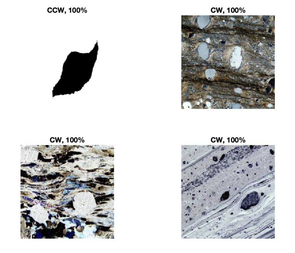
Examples of Some Heat Maps from our Training Set


Examples of BoW Using Naive Bayes
|
Examples of GANS
This is the code used to create the generator which make images from a noise vector and passes it to the discriminator
class Generator(nn.Module):
    '''
    Generator Class
    Values:
        z_dim: the dimension of the noise vector, a scalar
        im_chan: the number of channels of the output image, a scalar
        hidden_dim: the inner dimension, a scalar
    '''
    def __init__(self, z_dim=10, im_chan=1, hidden_dim=64):
        super(Generator, self).__init__()
        self.z_dim = z_dim
        # Build the neural network
        self.gen = nn.Sequential(
            self.make_gen_block(z_dim, hidden_dim * 4),
            self.make_gen_block(hidden_dim * 4, hidden_dim * 2, kernel_size=4, stride=1),
            self.make_gen_block(hidden_dim * 2, hidden_dim),
            self.make_gen_block(hidden_dim, im_chan, kernel_size=4, final_layer=True),
        )

    def make_gen_block(self, input_channels, output_channels, kernel_size=3, stride=2, final_layer=False):
        '''
        Function to return a sequence of operations corresponding to a generator block of DCGAN;
        a transposed convolution, a batchnorm (except in the final layer), and an activation.
        Parameters:
            input_channels: how many channels the input feature representation has
            output_channels: how many channels the output feature representation should have
            kernel_size: the size of each convolutional filter, equivalent to (kernel_size, kernel_size)
            stride: the stride of the convolution
            final_layer: a boolean, true if it is the final layer and false otherwise
                      (affects activation and batchnorm)
        '''
        if not final_layer:
            return nn.Sequential(
                nn.ConvTranspose2d(input_channels, output_channels, kernel_size, stride),
                nn.BatchNorm2d(output_channels),
                nn.ReLU(inplace=True),
            )
        else:
            return nn.Sequential(
                nn.ConvTranspose2d(input_channels, output_channels, kernel_size, stride),
                nn.Tanh(),
            )

    def forward(self, noise):
        '''
        Function for completing a forward pass of the generator: Given a noise tensor,
        returns generated images.
        Parameters:
            noise: a noise tensor with dimensions (n_samples, z_dim)
        '''
        x = noise.view(len(noise), self.z_dim, 1, 1)
        return self.gen(x)

def get_noise(n_samples, z_dim, device='cpu'):
    '''
    Function for creating noise vectors: Given the dimensions (n_samples, z_dim)
    creates a tensor of that shape filled with random numbers from the normal distribution.
    Parameters:
      n_samples: the number of samples to generate, a scalar
      z_dim: the dimension of the noise vector, a scalar
      device: the device type
    '''
    return torch.randn(n_samples, z_dim, device=device)
Code base taken from Coursera, modified to fit our needs
Results
SIFT with BoW (Naive Bayes)
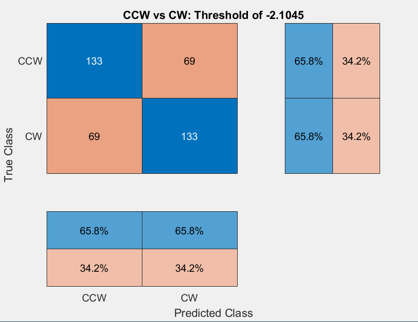
The Confusion Matrix displays which are the true values of the test data. Using the combined set of OG and Syn, the synthetic data yielded better results than the OG - due to the noisey features of the OG set.
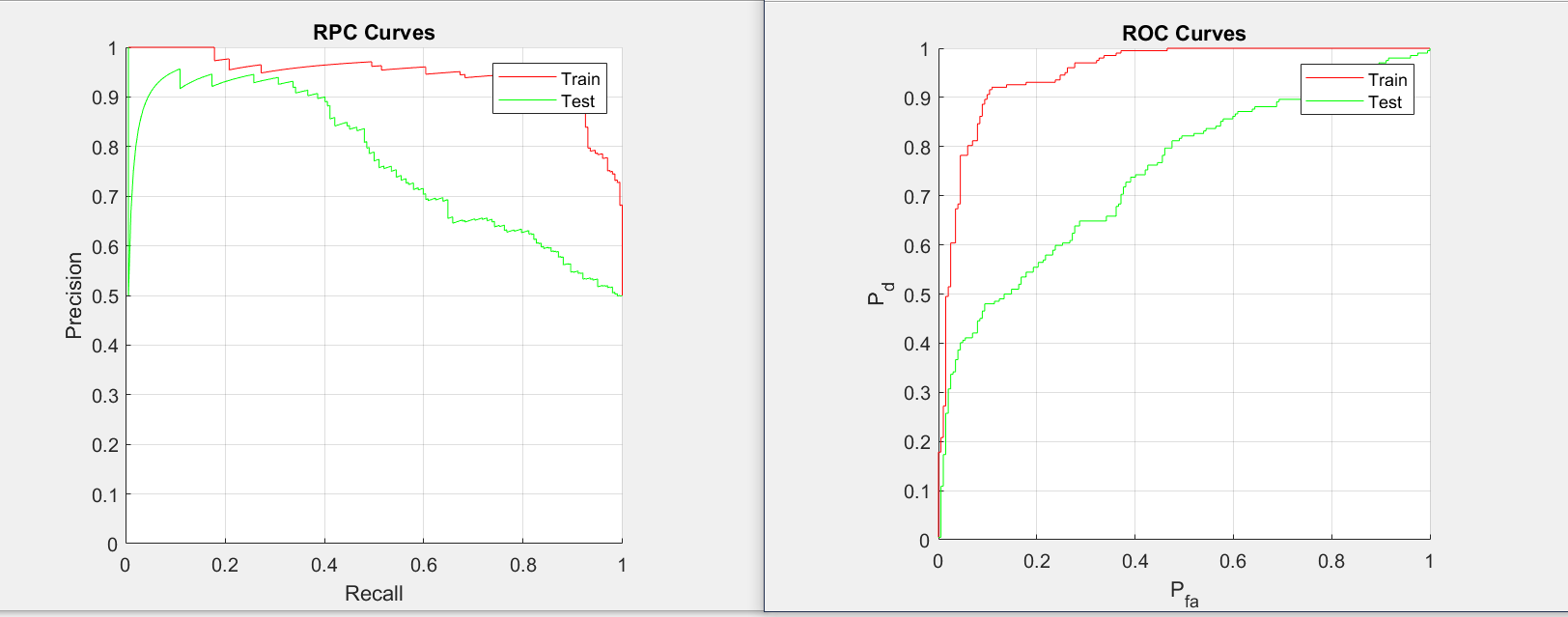
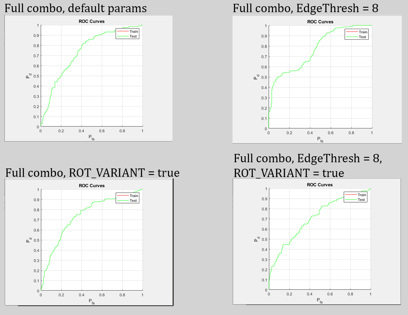
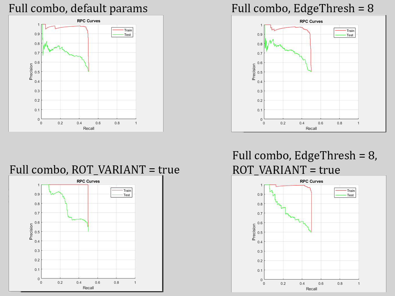
The curves shows the performance of classification model of all threshold
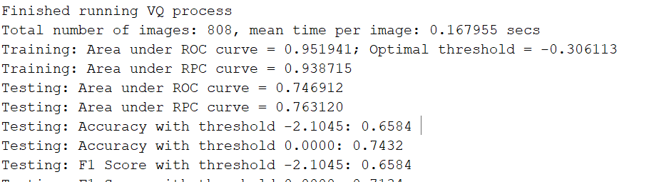
The results of the training, using the codebook at 800; these were the most optimal results out of all the tests ran.
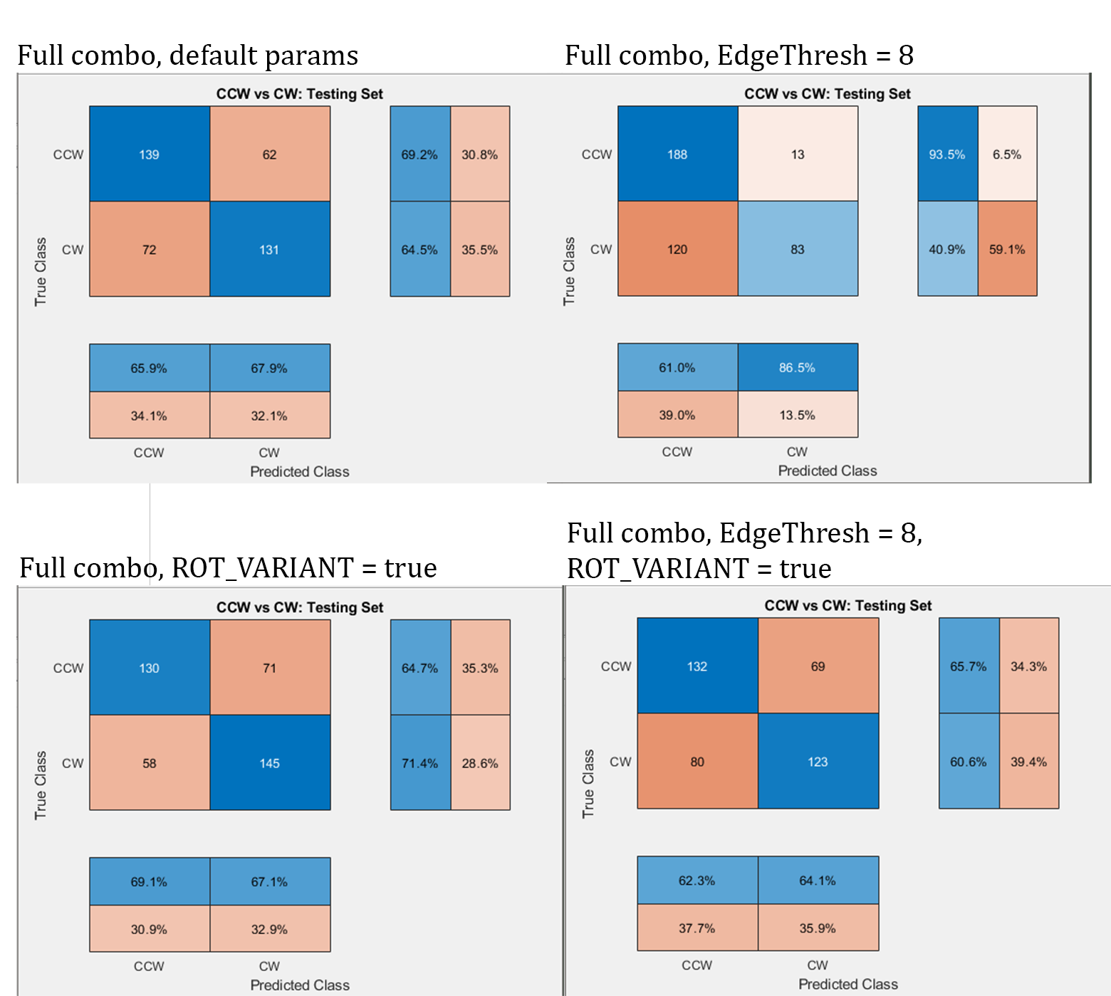
SIFT with Bag of Words (SVM)
All the following results for the BoW classifier (SVM model) were tested on the full combo dataset.
Parameters for best results achieved: ROT_VAR = false, EdgeThresh = 8
The edge threshold likely improved performance as features were closer to significant objects. The rotation variance parameter needs to be experimented with more before a conclusion can be drawn on its effectiveness.
CNN with SVM
This method used a CNN to extract features and fed that into a SVM classifier. We generated heat maps in order to pin point where the CNN was extracting features to allow for fine tuning to focus on the tails. This was somewhat successful with a combination of introducing synthetic images and tuning parameters to help with successful classification. There has not been any testing for classification bias, but this will be addressed in future work with these early promising results.

Image Classification using SVM

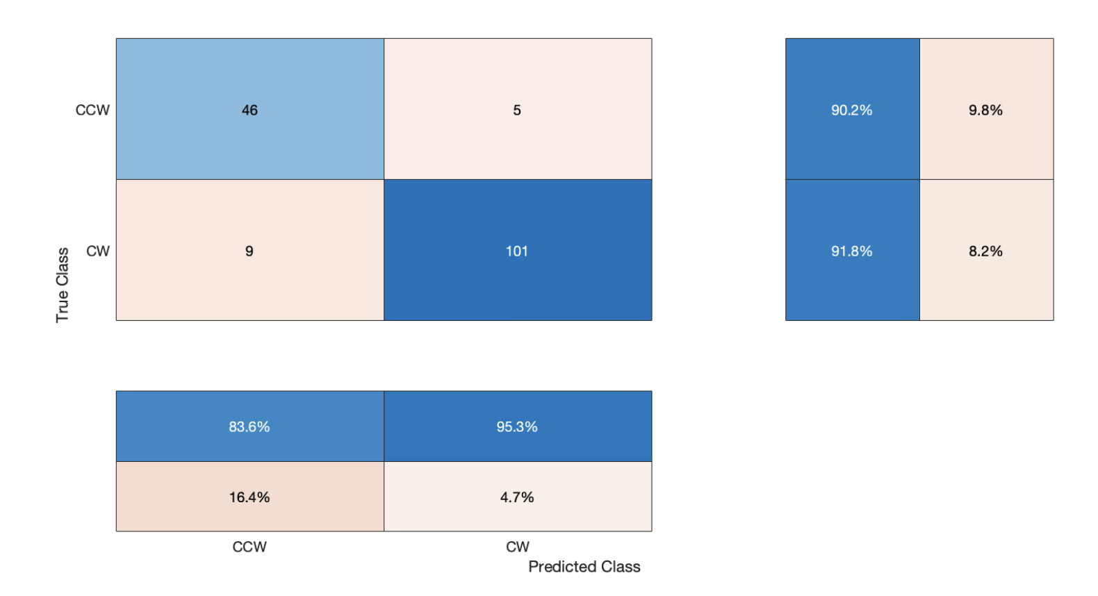
Accuracy (mean of diagonal of confusion matrix) is 0.9130
Avg F_Score is 0.9016
CNN with Transfer Learning
By using an already pretrained CNN, we added a new layer to GoogLeNet and the results were promising. While this hasn;t taken into account any bias, these preliminary results will give direction for future work. This method has fined tuned parameters and uses the larger 800 plus image set to get the best results we found.
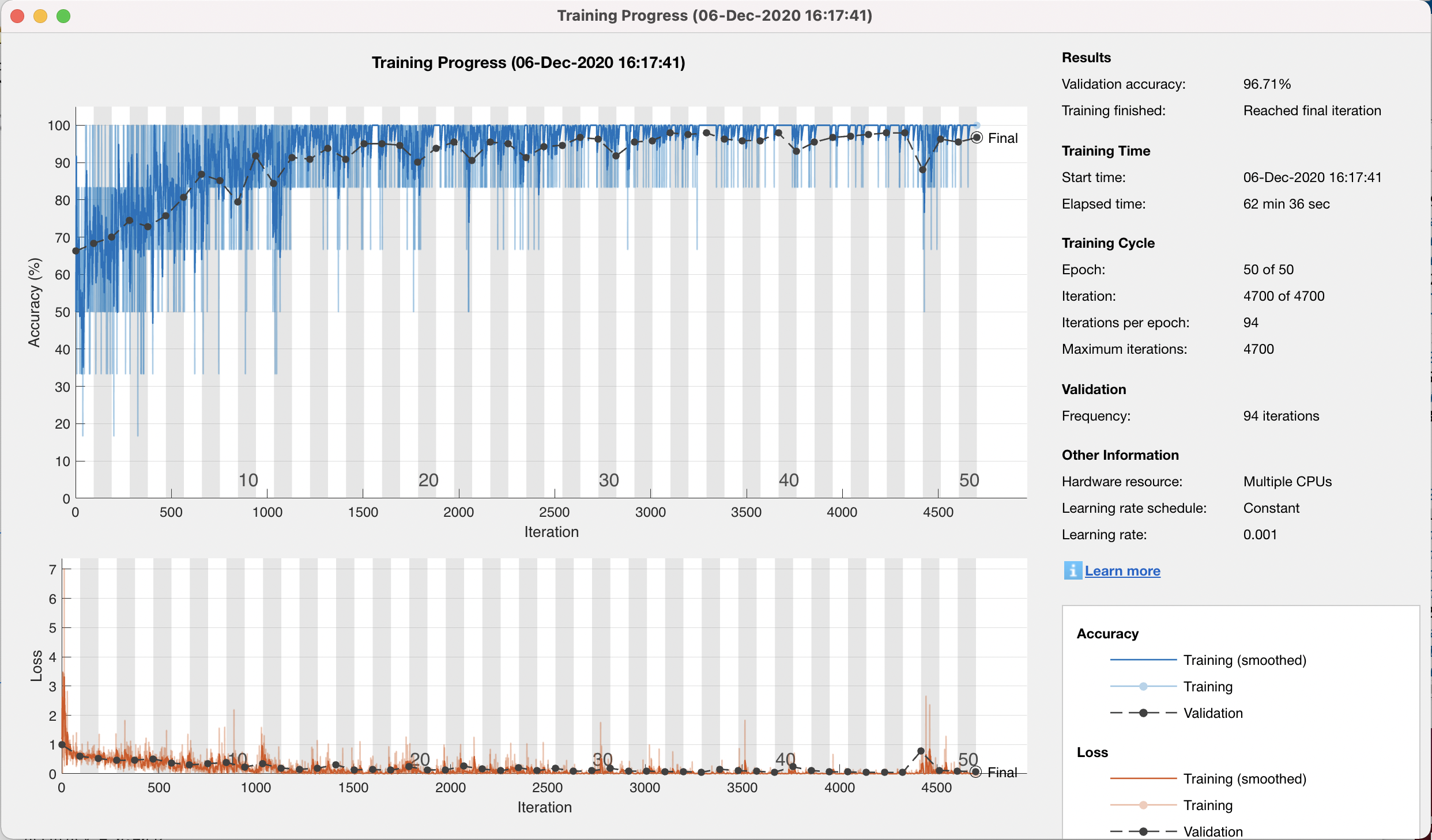
Accuracy/Loss graph of the training
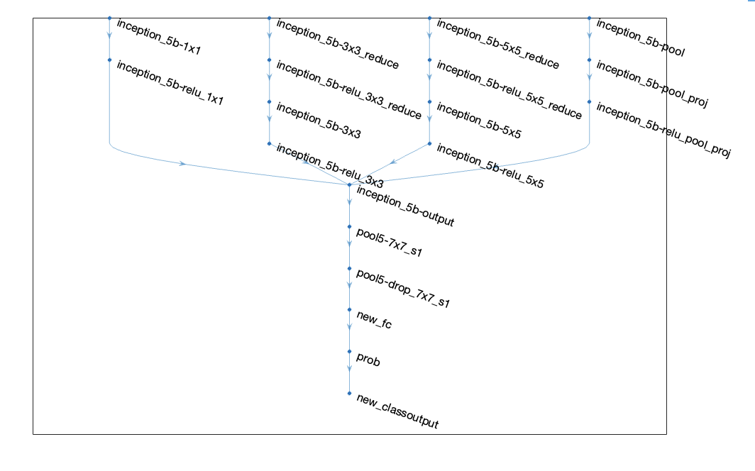
Additional Layer Added to GoogLeNet
Classification using Transfer Learning
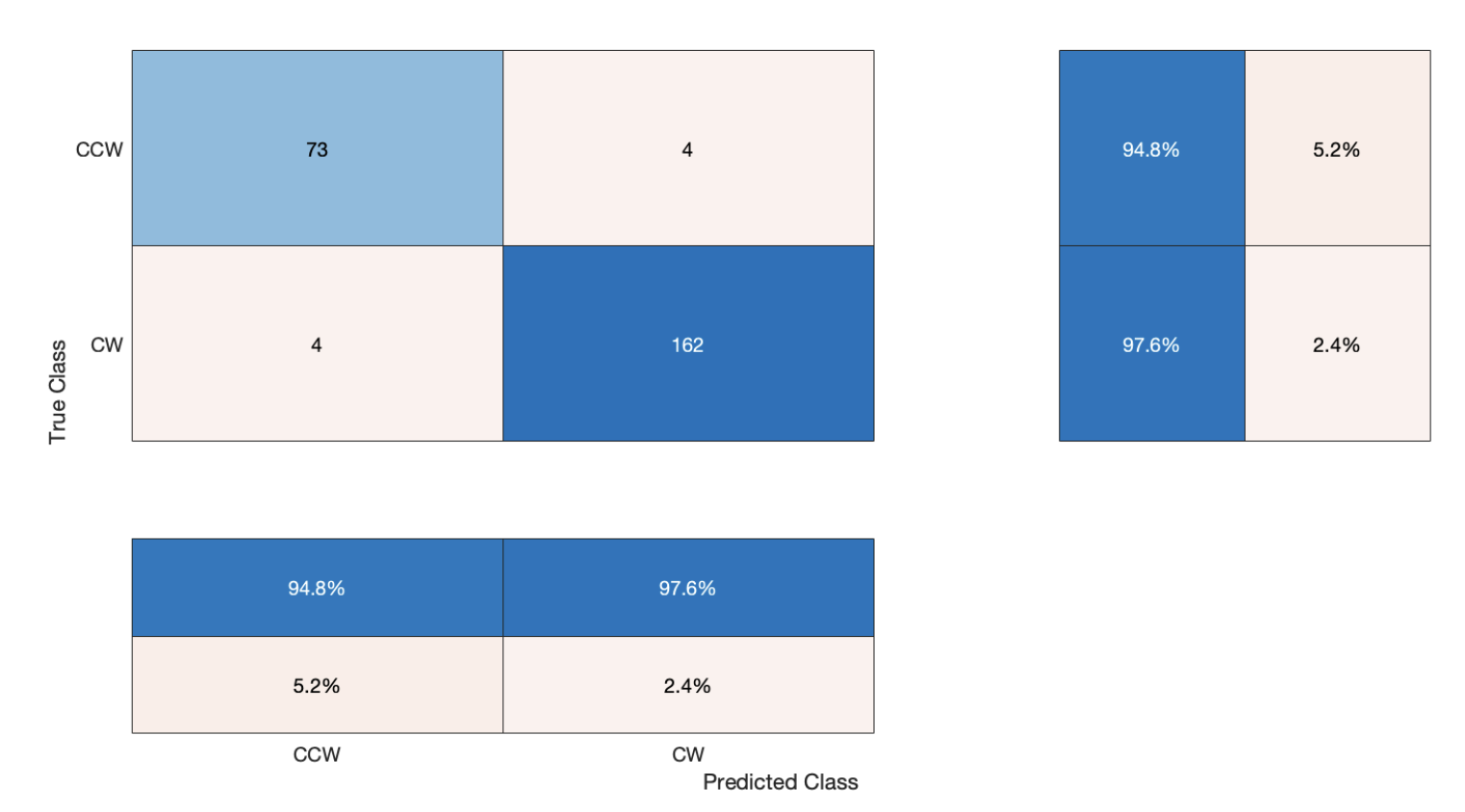
Accuracy (mean of diagonal of confusion matrix) is 0.9671
Avg F-Score is 0.9620
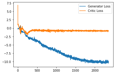
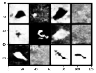
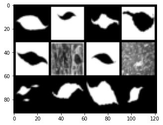
GAN
inA Generative Adversarial Network uses two Nueral Networks to produce data similar to the data it is trained with. During this time we were able to successfully generate 28x28 images that have goodfidelity and good diversity.
Example of Generator/Traing images. Top image block are the generated images and the bottom are the original data
Conclusion
Our experiments need to be repeated to ensure augmentation bias did not occur. Comparative experiments testing the transfer learning approach with GoogLeNet and the BoW classifier are also worth repeating with optimized parameters. Through the various methods and step taken, we have been able to significantly impact the outside research by giving feedback and data to allow time to be better spent on the more promising methods. This is also a proof of concept we can accomplish the task laid before us. We have observed that computer vision is capable of sheer-sense classification.