CS 470 : Project 1: Brain Machine Interface (BMI)

Above shows an illustration of the multi-channel positional layouts for 52 channels.
As our final project we chose to work on classyfing signals gathered from an Electroencephloography (EEG) device. The data set we chose was Mental arithmetic (003-2014) from the Graz University of Technology. The data we classified fell into two catagories: Mental Arithmetic, and Rest.
The data set consisted of recordings from eight subjects undergoing three or four trials each (Subjects one, two, and three underwent three trials each, while the other subjects underwent four). Using light emitters and light sensors, this data recorded brain oxygenation in fifty-two channels during these trials.
We started our project by reviewing the MatLab Machine Learning Onramp (https://matlabacademy.mathworks.com/R2019b/portal.html?course=machinelearning), as it was recommended to us due to having good information regarding the processing of one-dimensional data. Due to the issues surrounding the midpoint of the semester, we had a very slow start which hampered us later on as we had less time later to complete the project than hoped.
Method
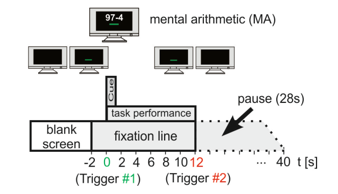
Above is an illistration of the experiment itself. The way the data was collected from the 8 subjects; each of the subjects were tasked with performing trials followed by consecutive rest periods for each trial. 2 seconds before the task started a green bar appeared on screen indicating the subjects get ready and the equipment would start recording. The subjects underwent 3-4 trials, each trial containing simple sequential subtraction problems. An example being 97 - 4, then 93 - 4 etc. After the experiment, the data complied to produce graphs depicting all 52 channels produced by the EEG. We then took that data and produced code to extract the listed 7 features below. By extracting 7 features from the 52 total channels, our end amount of features extracted was a 1092 total features.
Initially we did not use MatLab's built in function "fitcsvm" which did hamper our progress on the classification model. Below is the "fitcsvm statement.
%fitcsvm statement
mdl = fitcsvm(trainfeatures, trainclasses, 'Standardize', true, 'KernelFunction', 'rbf', 'OptimizeHyperparameters', auto);
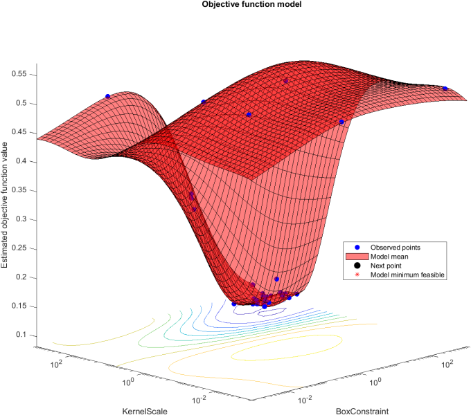
During the testing and training phase, seven subjects were used to train the svm and the one who was not included in the training was used to test the model. Initially the subjects being tested were chosen at random, but eventually cycled the testing position consecutively, through use of for loops. This change can attribute to an excessively long runtime. Below is an example plane of optimized hyperparameters for subject two,there are two parameters being tested for, KernelScale and BoxConstraint. It tests combinations (represented by blue dots) and finds the lowest estimated objective function value.
Features
Here is a list of features our code extracted, followed by a method of feature extraction:
Statistical:
- mean
- standard deviation
- skewness
- kurtosis
Hjorth descriptors:
- activity
- mobility
- complexity
%Feature Extraction Code
datachunk = readings(timestamps(b):timestamps(b+1),:);

            featureActivity = var(datachunk);
            dc1 = datachunk;
            dc2 = datachunk;
            for c = 2:size(datachunk,1)
                dc1(c,:) = datachunk(c,:) - datachunk(c-1,:);
            end
            featureMobility = std(dc1)/std(datachunk);
            for c = 3:size(datachunk,1)
                dc2(c,:) = datachunk(c,:) - 2*datachunk(c-1,:) + datachunk(c-2,:);
            end
            featureFF = (std(dc2)/std(dc1))/(std(dc1)/std(datachunk));
            featureMean = mean(datachunk);
            featureKurtosis = kurtosis(datachunk);
            featureSkewness = skewness(datachunk);
            featureStd = std(datachunk);
Results
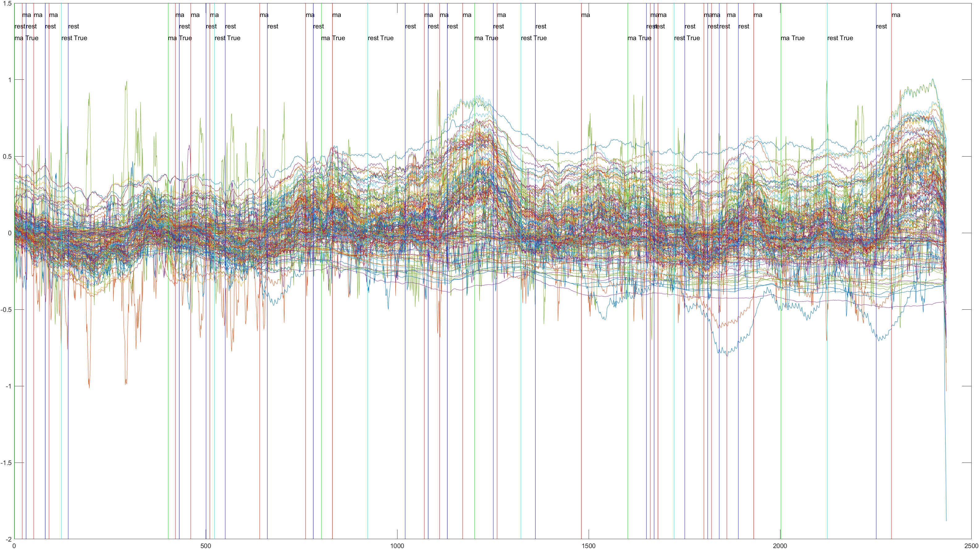
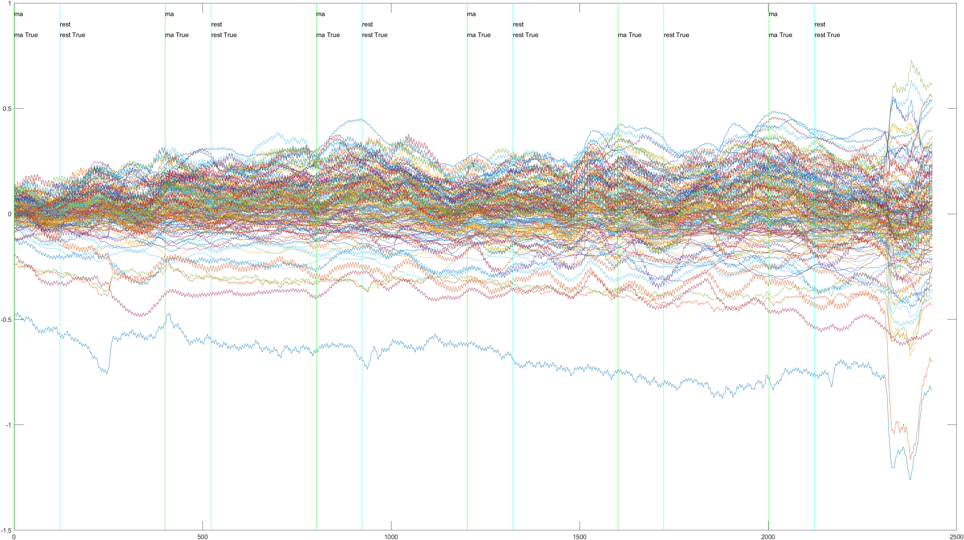
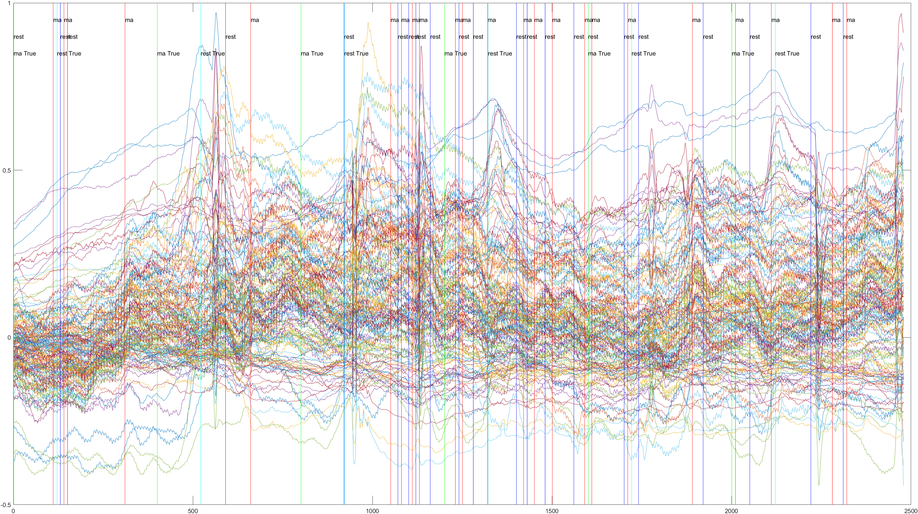
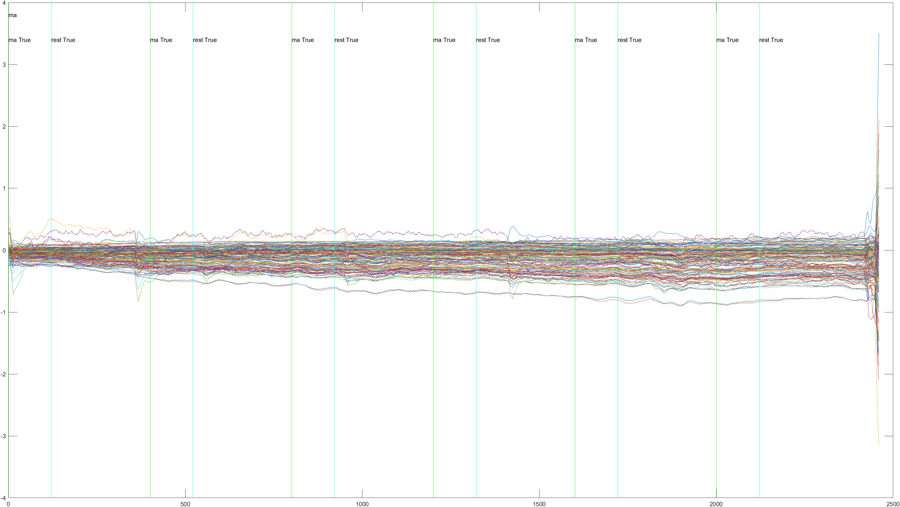
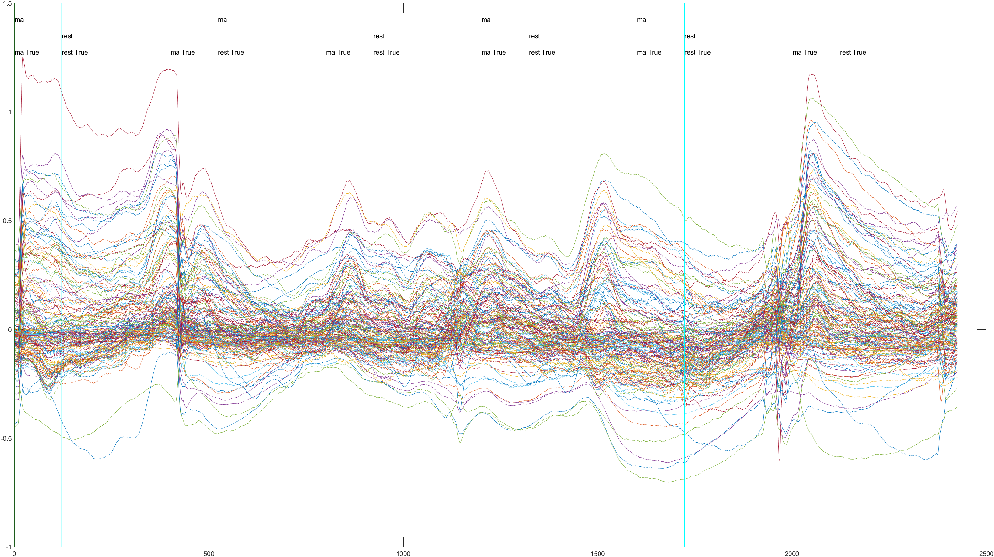
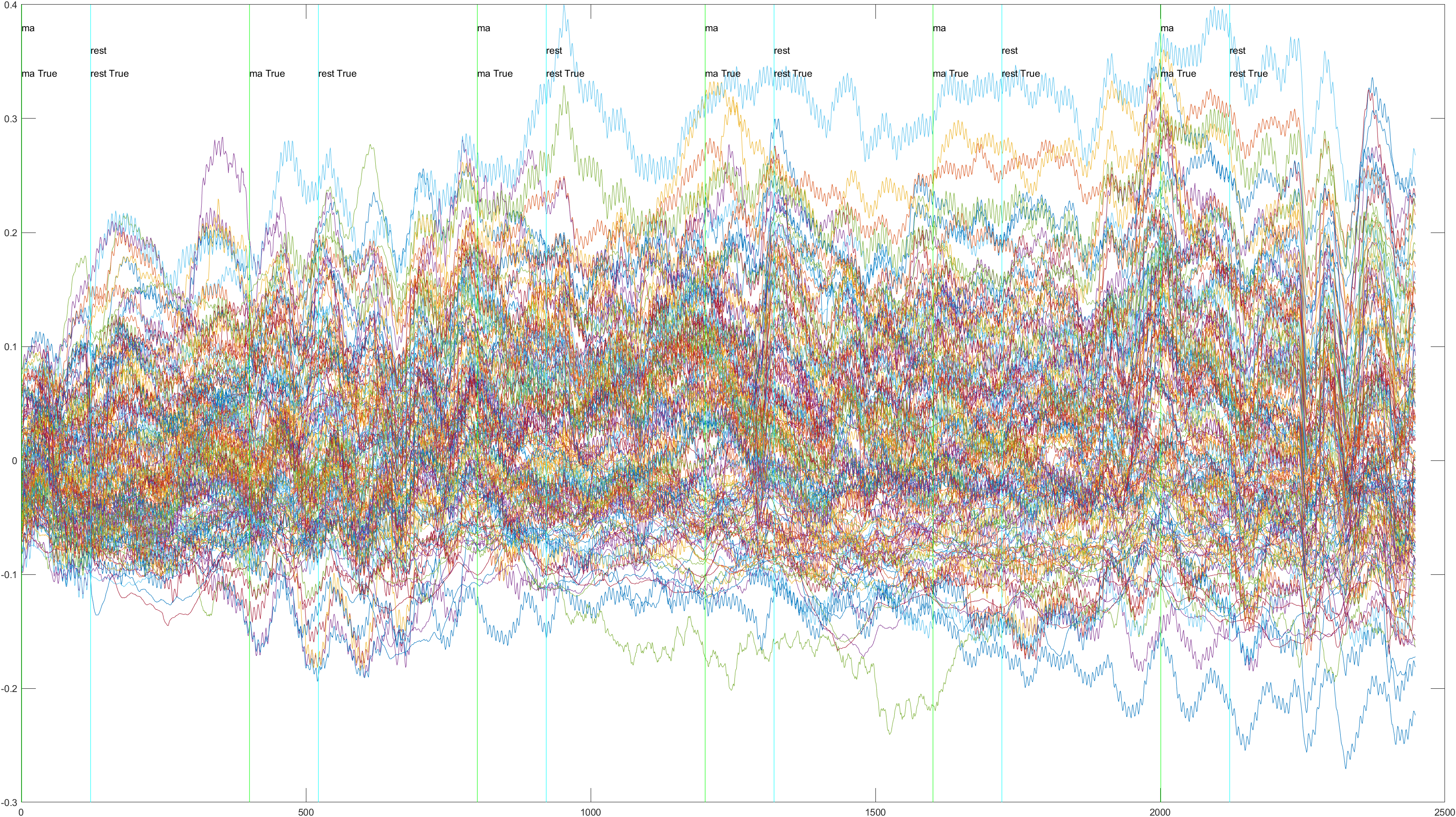
Here is the graph showing all 52 channels produced by Subject 2 during trial 1, without the sliding feature implimented.

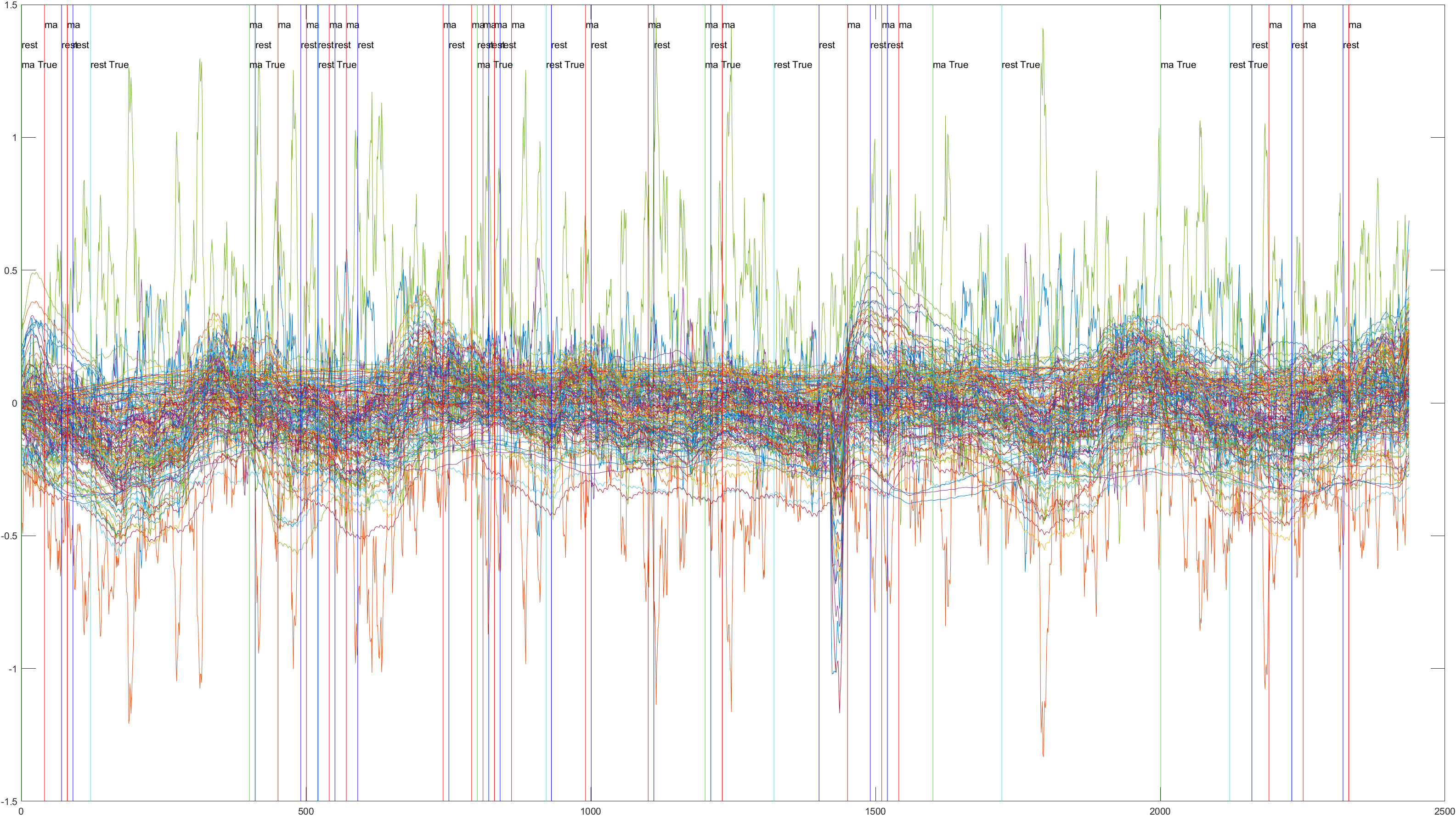
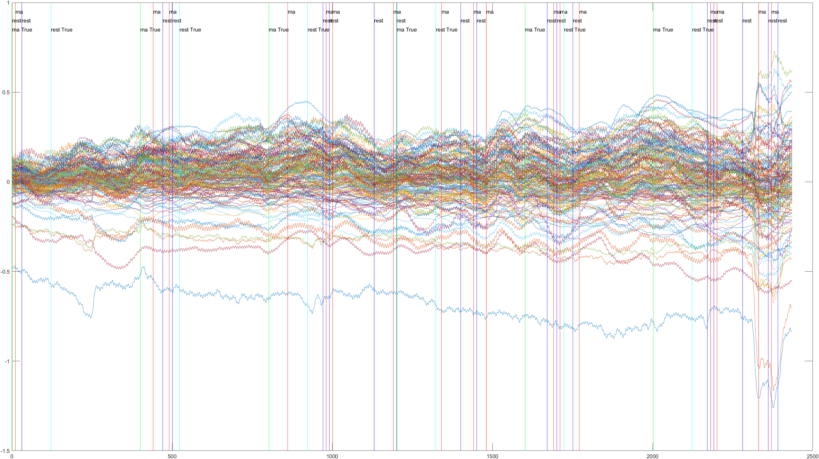
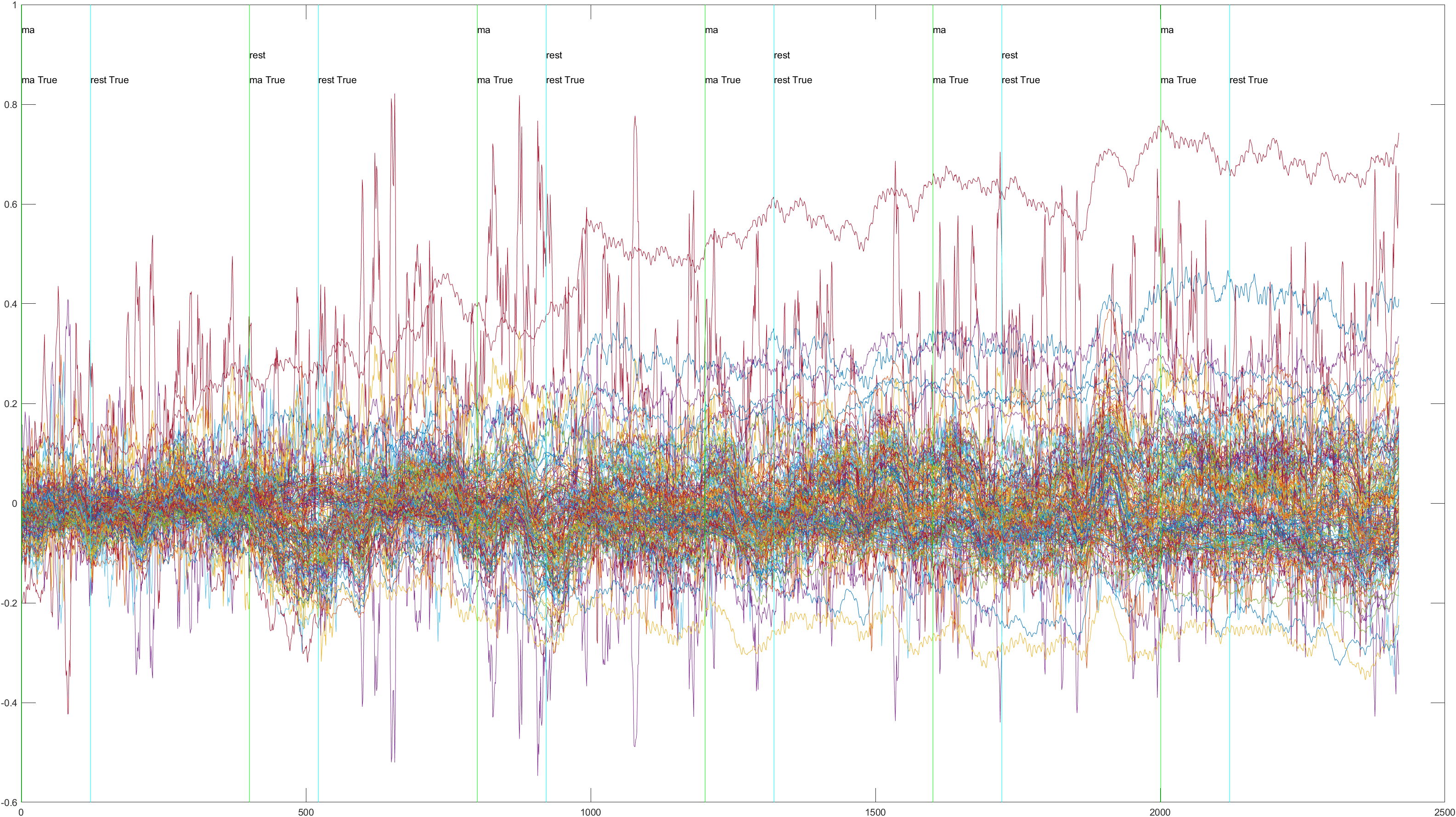
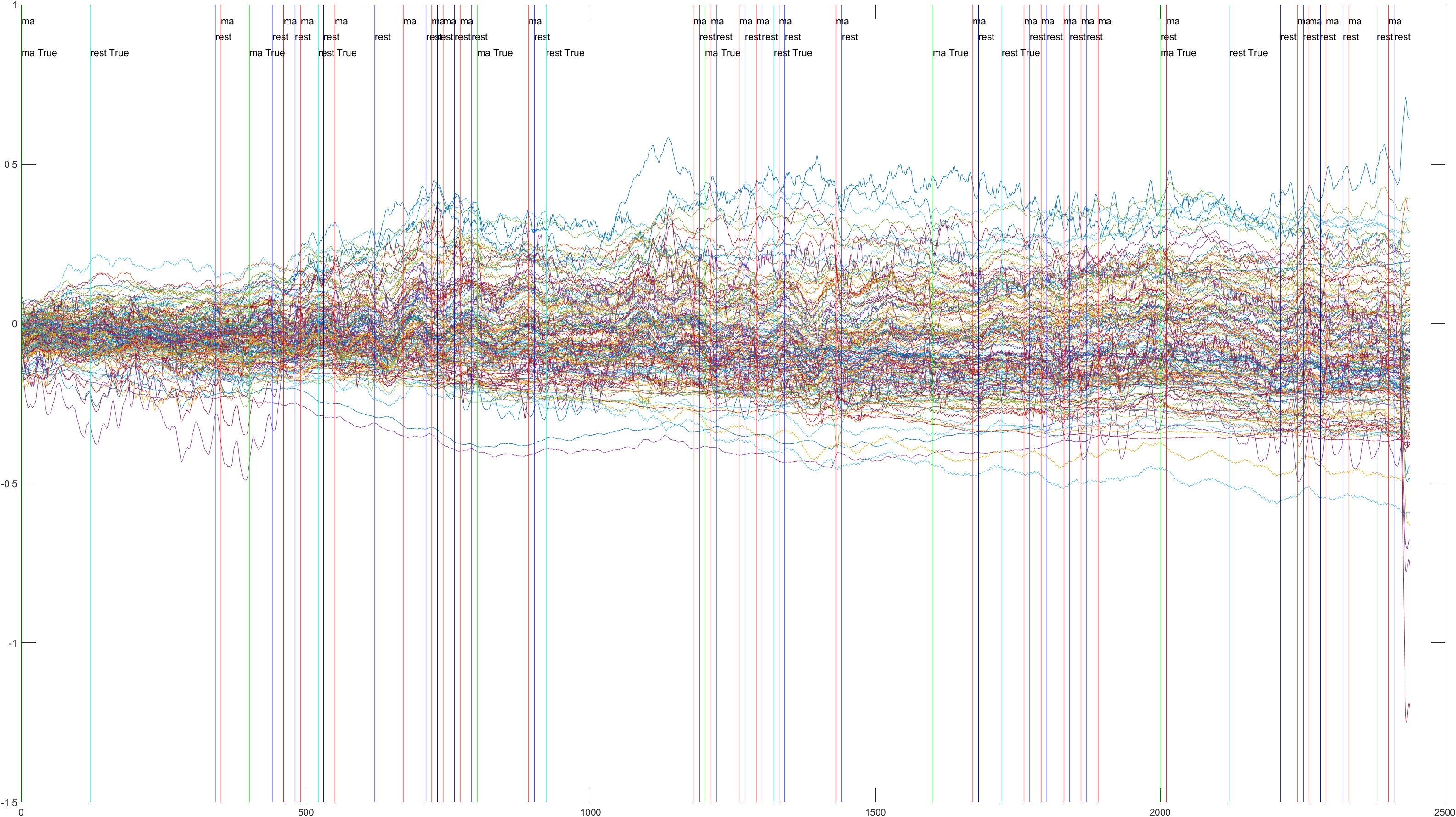
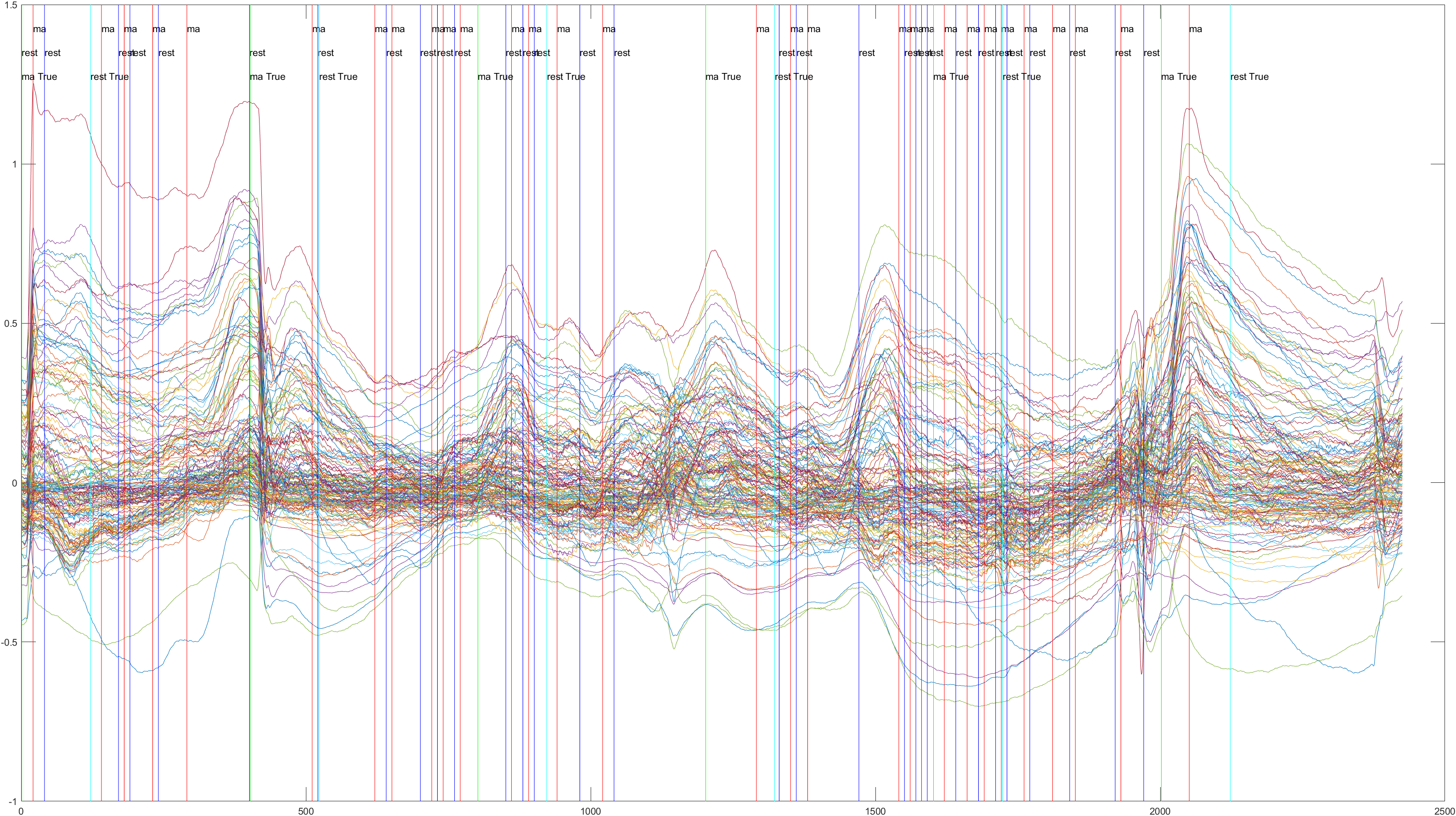
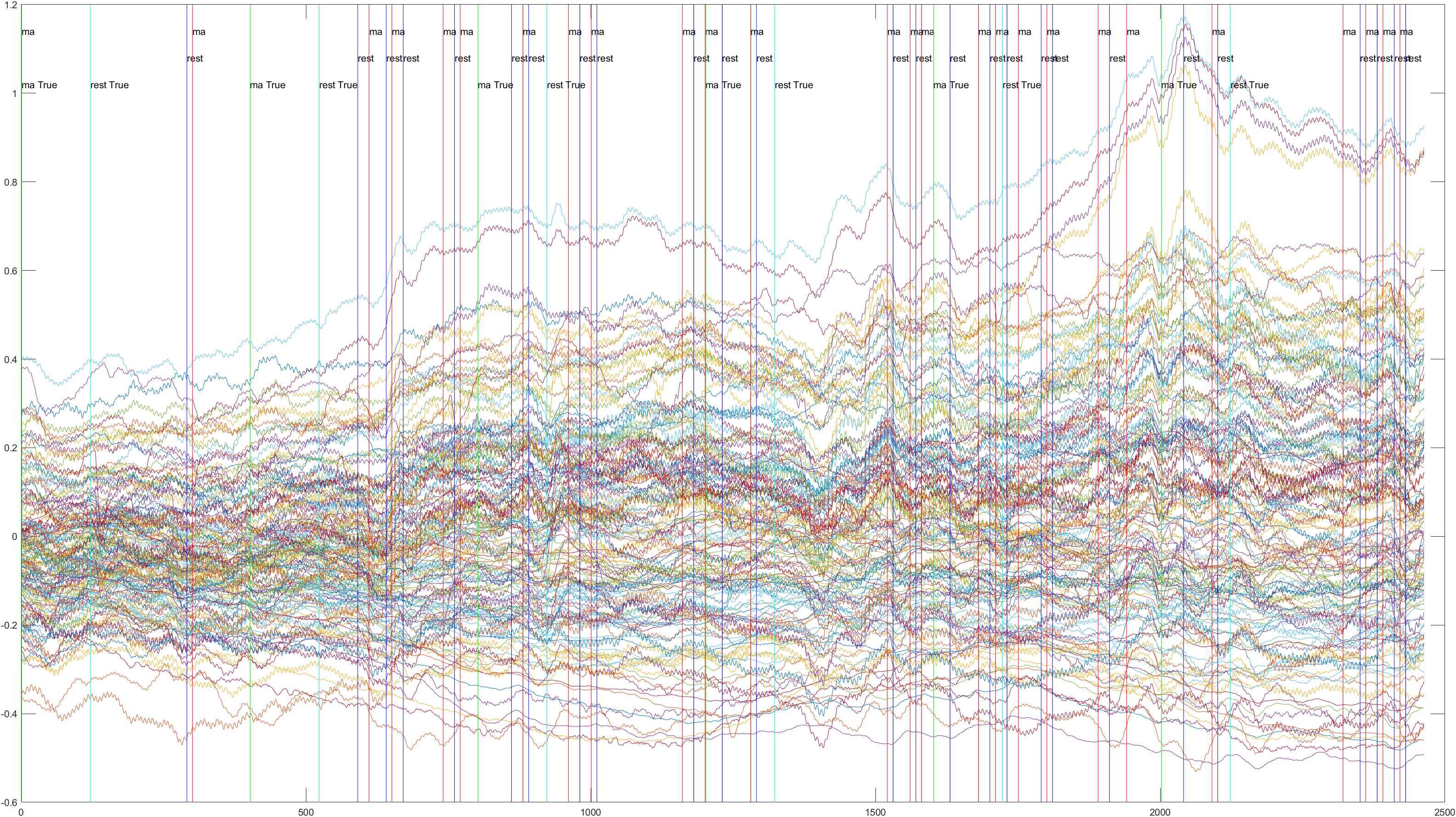
Subject 2 trial 1, with the sliding window implimented

A table containing all subject and their (sliding/non-sliding) trials
| Subject # | Total Trials | Trial 1 | Trial 2 | Trial 3 | Trial 4 | ||||
|---|---|---|---|---|---|---|---|---|---|
| Subject 1 | 3 |  Non-Sliding |
 Sliding |
 Non-Sliding |
 Sliding |
 Non-Sliding |
 Sliding |
n/a |
n/a |
| Subject 2 | 3 |  Non-Sliding |
 Sliding |
 Non-Sliding |
 Sliding |
 Non-Sliding |
 Sliding |
n/a |
n/a |
| Subject 3 | 3 |  Non-Sliding |
 Sliding |
 Non-Sliding |
 Sliding |
 Non-Sliding |
 Sliding |
n/a |
n/a |
| Subject 4 | 4 |  Non-Sliding |
 Sliding |
 Non-Sliding |
 Sliding |
 Non-Sliding |
 Sliding |
 Non-Sliding |
 Sliding |
| Subject 5 | 4 | 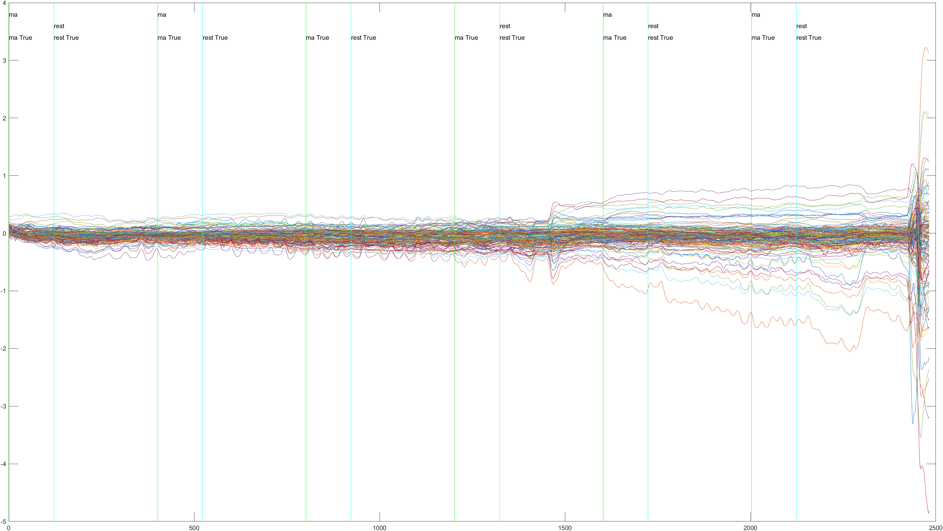 Non-Sliding |
 Sliding |
 Non-Sliding |
 Sliding |
 Non-Sliding |
 Sliding |
 Non-Sliding |
 Sliding |
| Subject 6 | 4 |  Non-Sliding |
 Sliding |
 Non-Sliding |
 Sliding |
 Non-Sliding |
 Sliding |
 Non-Sliding |
 Sliding |
| Subject 7 | 4 |  Non-Sliding |
 Sliding |
 Non-Sliding |
 Sliding |
 Non-Sliding |
 Sliding |
 Non-Sliding |
 Sliding |
| Subject 8 | 4 |  Non-Sliding |
 Sliding |
 Non-Sliding |
 Sliding |
 Non-Sliding |
 Sliding |
 Non-Sliding |
 Sliding |
| Subject # | Total Trials | Trial 1 | Trial 2 | Trial 3 | Trail 4 | ||||
Overall our result, were recorded as follows:
For no sliding window, the Average Accuracy is 0.8550, the Average Fscore is 0.9399, the Accuracy STD is 0.0917, and Fscore STD is 0.0526.
For sliding window, the Average Accuracy is 0.5090, the Average Fscore is 0.7607, the Accuracy STD is 0.0596, the Fscore STD is 0.0662.
Conclusions
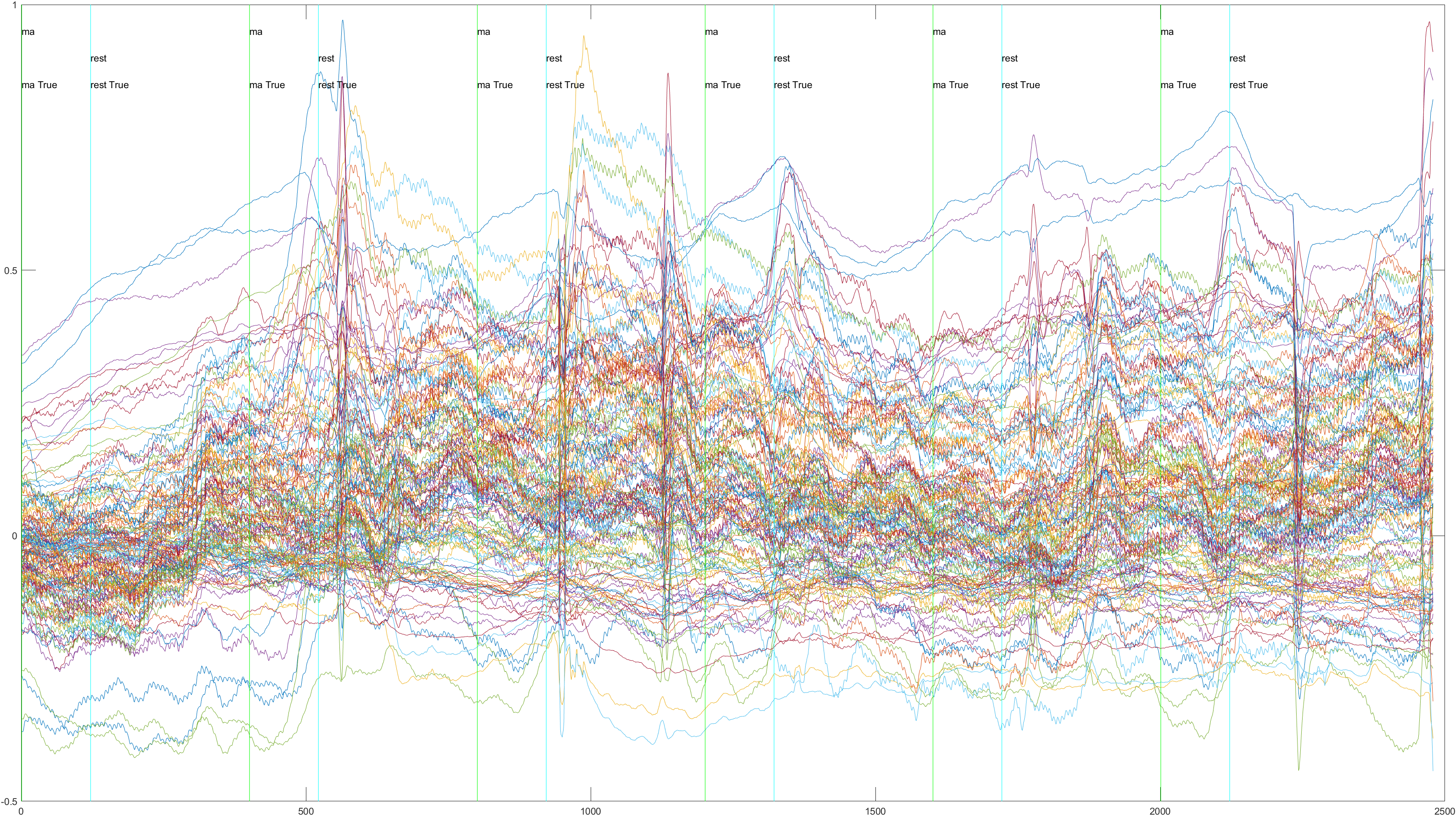
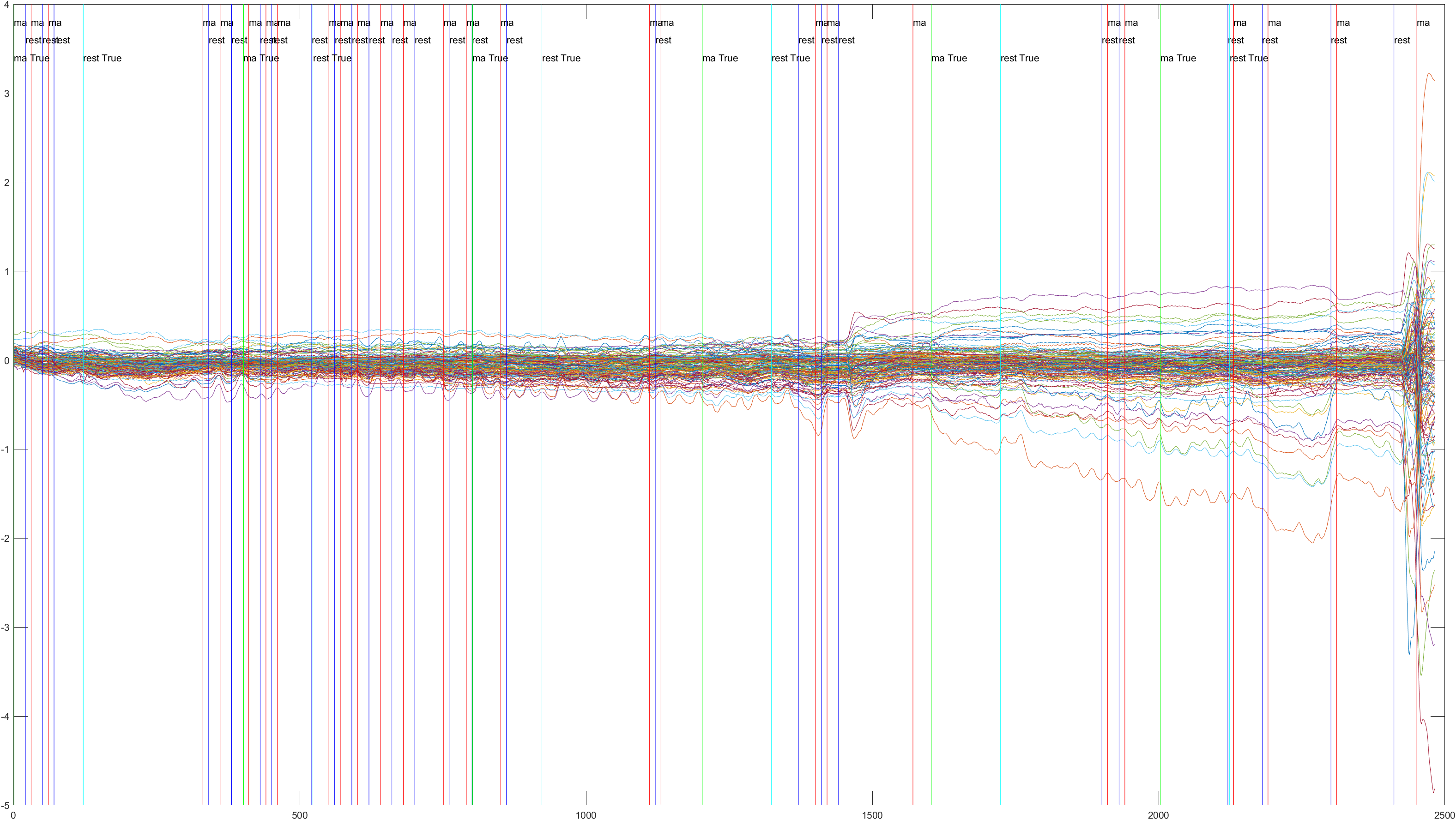
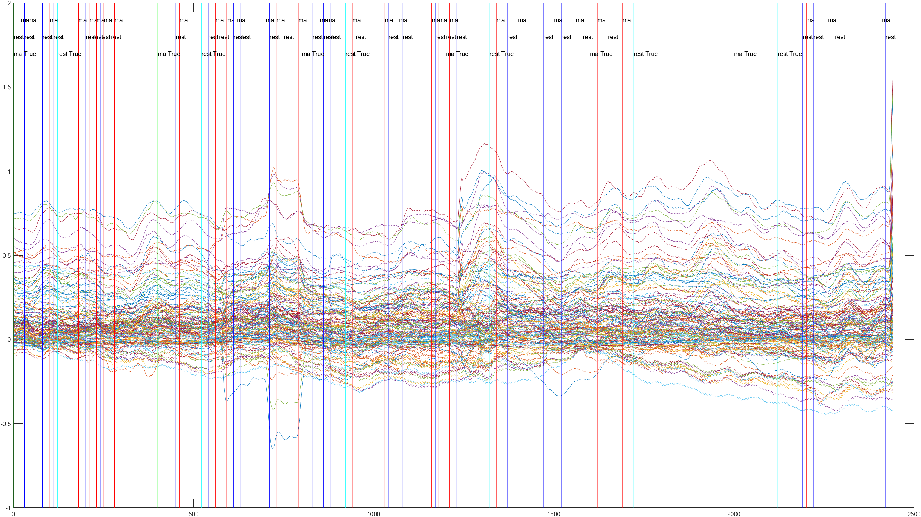
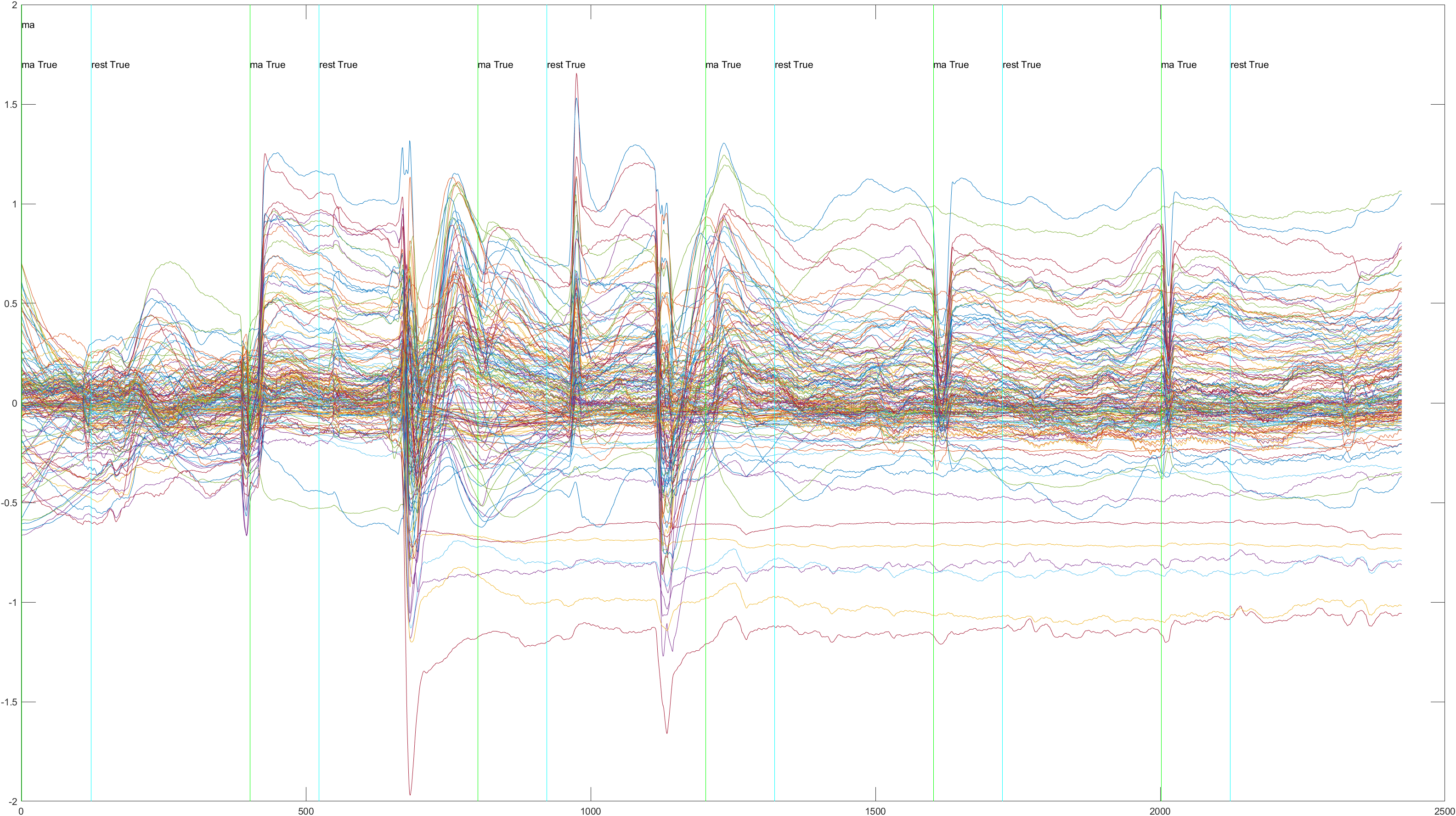
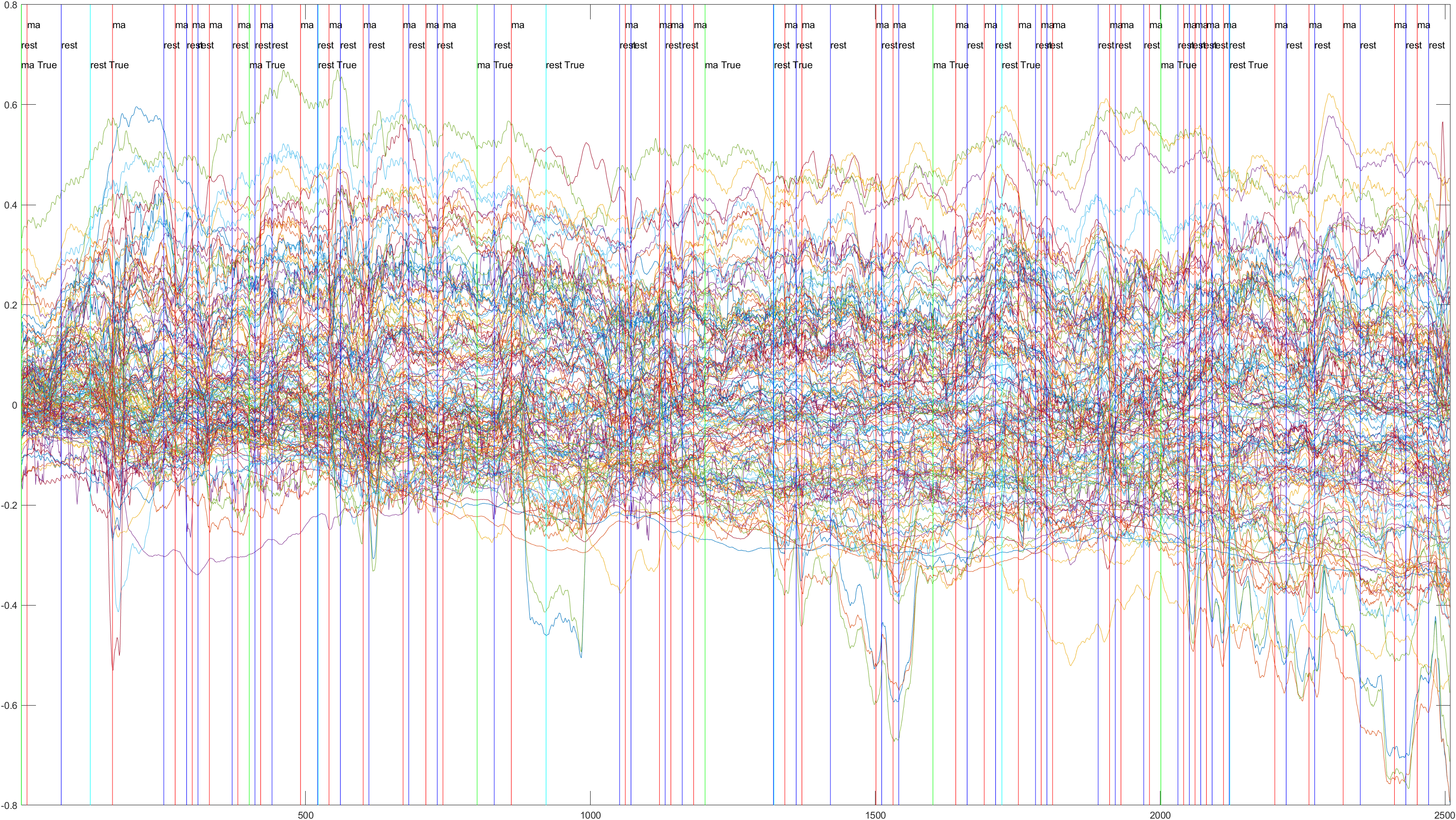
The issues we had with the Sliding Window approach, I think may have had to do with noise in the data. It's difficult to detect noise in EEG data as it is much less intuitive than image data. For example, in the Subject 6, Trial 4 data we can see a much lower reading at the beginning of the data, followed by a large spike at the end, which was present in many of the trials. We're not sure if this is noise, or legitimate data relating to waiting prior to the experiment and moving just afterwards. In addition, we were not able to find a good window size to scan across the data with, which I believe meant that we had many radically different samples that the classifier could not properly train on. In order to remedy this, a larger dataset, designed for this project and monitored for noise, would be helpful. Unfortunately we were unable to gather data ourselves and were limited to premade datasets findable online. In addition, we saw a large discrepancy in accuracy between runs, even without implementing the sliding window. When used as a test, Subject 3, the highest, had an accuracy of .9444, while Subject 6, the lowest, had an accuracy of just .6875. This may be indicative of noise in Subject 6's data, but it may just be discrepancies between patients, or a different mindset upon exposure to the test on Subject 6's part. More research is needed to more accurately determine the differences in brain oxygenation between different subjects under the same conditions. Still, with refinement, these findings show promising potential for using brain oxygenation to classify mental activity. This, coupled with more traditional EEG readings, could lead to more accurate, consistent results.