CS 470 Final Project

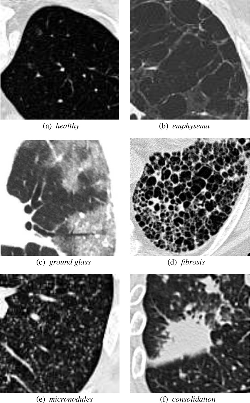
Interstitial lung diseases are a collection of diseases which cause scarring of the lung tissue. In order to diagnose these diseases radiologists must scour a series of CT scans for a patient. With the use of machine learning the time of radiologists could be saved by allowing them to validate results returned from a machine learning algorithm allowing it to do all the heavy lifting. In order to carry out this vision our team set out to design two distinct classification methods for CT scans in order to compare their efficacy and accuracy. Those two distinct classification methods were a Regional-CNN and a CNN which employed the use of sliding window classification. The results of the R-CNN leave much to be desired because obtains an average precision of 0% on most patients with some patients getting around 2% - 3% average precision. The highest ground glass average precision was 10% and fibrosis was 22%. This data was gathered with fifteen patients which equates to about 130 images in the training set. Increasing the amount of classes in the dataset also decreased the accuracy so the data was tested on only two classes.

Introduction to R-CNN

An R-CNN is very similar to a CNN the difference is that a R-CNN takes an image and divides into a fixed number of slices. These fixed number of slices are known as region proposals. These regions are cropped and resized and fed into the CNN. After they are classified the bounding boxes are refined with the use of SVM.

R-CNN workflow. Source: R-CNN workflow

Designing an R-CNN

The initial stages of designing the R-CNN consisted of structuring the data for proper format. The MATLAB documentation specified that the data be specified in table format with the first column being a vector of file names, and the other subsequent column names being the location of the ROI. Each subsequent column would represent the class being identified. The sizes of columns must be equal to each other so many columns would have empty observations because they only contain one class.

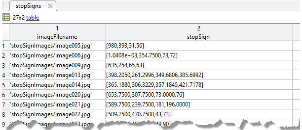
Training data structure for single class identification. Source: Train R-CNN

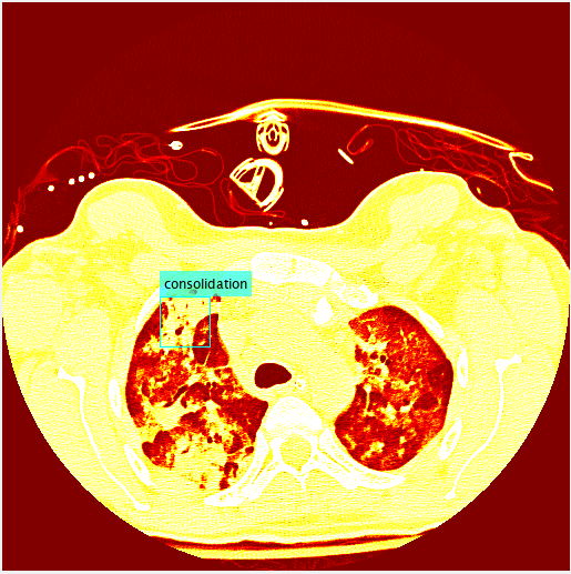
Another specification for training the R-CNN classifier required the images to be in a format recognized by imread(). Since the CT slices were dicom images their pixel coordinates were described in Hounsfield Units or (HU). HU pixel values typically range from -1000 to 1000. So in order to create valid data for the R-CNN the images needed to be converted from HU to valid RGB pictures. Luckily there was functionality for this already in place in the project.

Bounding box for a single class mapped to RGB.

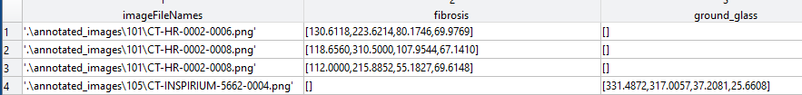
The structuring of this data initially proved to be challenging single class identification was simple because each image corresponded to the single class. However, when converting the classifier to multiclass there had to be empty observations for the other classes. This problem was solved with the use of cell arrays which are very flexible.

Training data structure for multi class identification.

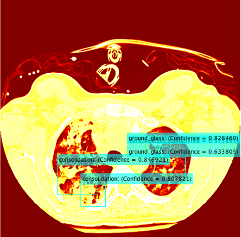
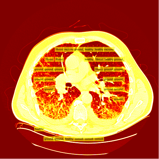
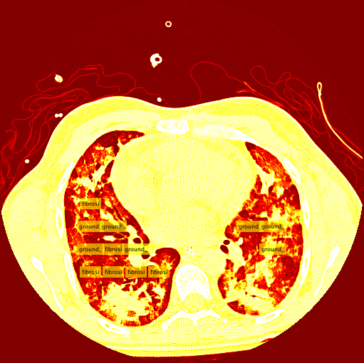
After the data was structured for training it next needed to be segmented for creating valid training sets. Each patient had a series of CT slices within each folder. In order to create a valid training and test set of this it had to recognize these folders. This meant restructuring my code in order to create folders for each patient to store each slice in. From here the data could be recognized by distinct patients rather than a collection of arbitrary CT slices. From here leave one out validation could be applied with relative ease. With valid training and test sets created the R-CNN could now make predictions on the data.

R-CNN Prediction on a CT slice

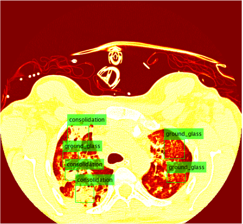
Ground truth boxes

The settings that were used for the R-CNN did not deviate far from the defaults specified within the documentation.


		% CNN -> R-CNN
		net = resnet18;
		numClasses = numel(diseaseLabels) + 1;
		lgraph = layerGraph(net);
		% Remove the the last 3 layers. 
		layersToRemove = {
			'fc1000'
			'prob'
			'ClassificationLayer_predictions'
			};

		lgraph = removeLayers(lgraph, layersToRemove);

		% % Define new classfication layers
		newLayers = [
			fullyConnectedLayer(numClasses, 'Name', 'rcnnFC')
			softmaxLayer('Name', 'rcnnSoftmax')
			classificationLayer('Name', 'rcnnClassification')
			];

		% % Add new layers
		lgraph = addLayers(lgraph, newLayers);

		% % Connect the new layers to the network. 
		lgraph = connectLayers(lgraph, 'pool5', 'rcnnFC');

The basic workflow for creating an R-CNN was using one of the pretrained models and replacing the last three layers with a fullyConnectedLayer, softmaxLayer, and finally a classificationLayer. As for the training the defaults did not stray too far away from the defaults mentioned in the MATLAB documentation either, some variables were tweaked but not too many.

		
			options = trainingOptions('sgdm', ...
			'MiniBatchSize', 128, ...
			'InitialLearnRate', 1e-3, ...
			'LearnRateDropFactor',0.2, ...
			'LearnRateDropPeriod', 5, ...
			'MaxEpochs', 15, ...
			'ExecutionEnvironment', 'gpu');

			rcnn = trainRCNNObjectDetector(trainDataTable, lgraph, options, ...
			'NegativeOverlapRange', [0 0.3], 'PositiveOverlapRange',[0.4 1])

R-CNN Results

The results for the R-CNN were unimpressive, in most training the results of average precision for each patient was 0%. There were a small percentage of patients which had an average precision of around 2% - 3%. The highest precision for ground glass was 10% and 22% for the fibrosis class. These results were on 15 patients which unfortunately takes a very long time due to leave one out validation of the data.

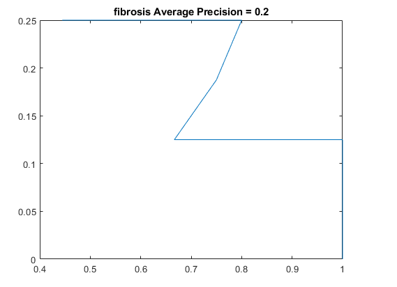
$images\fibrosis precision recall plot$

Fibrosis precision recall plot (x: precision y: recall)

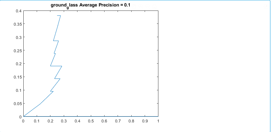
Ground glass precision recall plot (x: precision y: recall)

Increasing the amount of patients gives a minor improvement on the data overall but the time that it takes to run dramatically increases. Overall the results leave much to be desired and it is currently unclear if it is faulty code which is leading to these results, lack of training data or a combination of both.

Conclusion

The R-CNN quantitatively was a failure, as of right now it is uncertain whether this is a bug within the code or a lack of training data. Assuming it is not a bug which is causing these low recognition rates there are some areas of the project which could be affecting the accuracy of the classifier. The most likely of which would be the conversion from Hounsfield units to RGB. There is certainly some data loss when applying this conversion and if there was a better alternative to conversion then this could improve accuracy.

The Sliding Window Method

The sliding window method consists of taking an image and iteratively "sliding" the clasifier over the entire image starting from the top left and moving to the top right, then moving down a row and restarting at the left. Unlike the R-CNN, the sliding window system takes patches and feeds them into a seperate, external classifier. This external classifier is solely responsible for classifying patches fed to it while the sliding window is an algorithm that intelligently finds the best patches to feed to the classifier.

Intelligent Patch Search Algorithm

A tough decision I had to make was determining which patches to send to the classifier, and the best way to get them. At first I was considering training an additional class of images, the background class. This would entail the sliding window to send every patch to the classifier, and ignore patches that were classified as backgrounds. In retrospect, this would have been the smarter decision. The second potential method was using a "threshold" to determine which patches to send to the classifier in the first place. I ended up using this method, and my threshold was, for the most part, smart enough to correctly find the lung in a CT slice.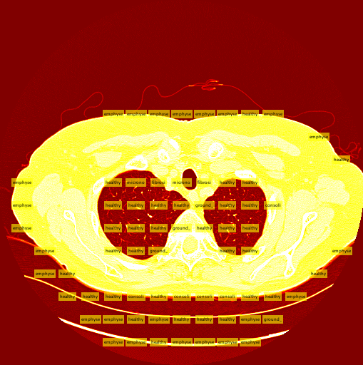

The thresholding system is still imperfect due to the simplicity of the algorithm. A few patients have more vastly different slice backgrounds, and as a result the thresholding system becomes totally ineffective for those slices. Still, the vast majority of patient slices work well with the threshold. The classifier used was a pretrained alexnet network that I modified to detect diseases in image patches from the training data. I performed a similar training algorithm to the Matlab transfer learning with some changes to get the best accuracy possible. The settings I used to train and determine the accuracy of are shown below.

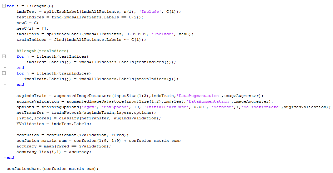A special consideration I needed to take to get an accuracte estimate of the classifer is bias in the testing data. Put simply, training and testing a classifier using the same images creates a strong bias that makes for an apparently much more accurate classifier. The solution is a method called "leave one patient out cross validation." Removing this bias can be possible if you train on n-1 patients and test on a single patient, repeating n times and picking a different "leave out patient" each iteration.

Results

My sliding window and classifier worked decently, and for the most part turned out okay results. However, there was still big room for improvement. Here is the "confusion matrix" of my classifier made using leave one patient out cross validation. A confusion matrix is a table depicting where the classifier is working and where it is not, but it can be used with any data matrix. I only I had just a bit more time to fully take advantage of the data is table has to offer. (insert confusion, results about images)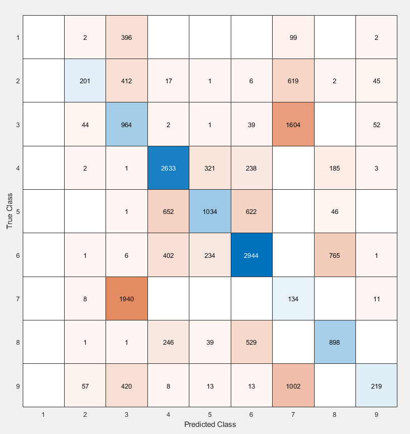

1-bronchiectasis, 2-consolidation, 3-emphysema, 4-fibrosis, 5-ground glass, 6-healthy, 7-macronodules, 8-micronodules, 9-reticulation

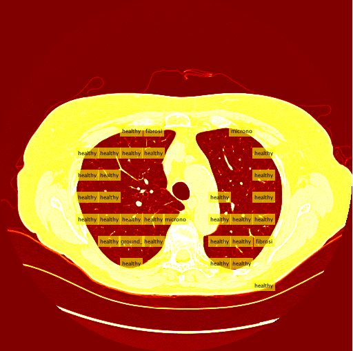
Healthy Lung Example:

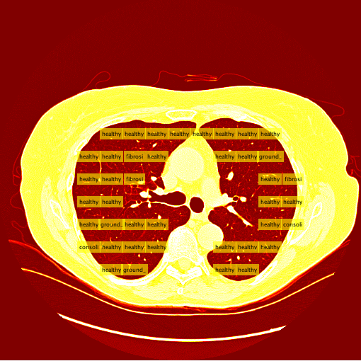
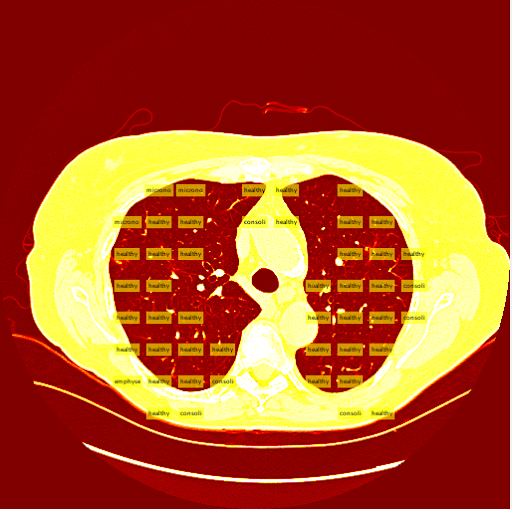
Ground Glass Lung Example:

Conclusion

If I were to redo the project, I would train a background class and use that to create a perfect lung finder. I would do this by taking the non-lung area patches from data that has a proven track record of working well with my current algorithm. This would include the background and parts of the body that is not a lung.

I would also like to only highlight patches of disease that are actually diseased. Classifying sixty percent of a lung as ground class would outscale whatever else the classifier returned, snd therefore only the ground glass flags would be raised for the user to. Next, I would remove some troublesome data such as patients with limited data. Limited data patients often result in a perfect or zero accuracy. I may even remove a disease all together if I couldn't get the accuracy up.

ILD Classification Nicolas Ginocchio, Jason Hubbs, Tairyn Addison

CS 470 : The Classification of Interstitial Lung Disease

Introduction to R-CNN

Designing an R-CNN

R-CNN Results

Conclusion

The Sliding Window Method

Intelligent Patch Search Algorithm

Results

Conclusion