CS 470: Preventing wildfires using point cloud segmentation and forest data extraction
Introduction:
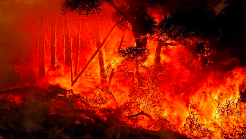
Kincade Fire
The main objective of our project was to analyze forests to manage the spreading of wildfires. By rapidly and more accurately estimating above ground biomass we can help prevent wildfires like Tubbs and Kincade Fire. We took two different approaches, machine learning using Lidar 360, Matlab and 3 python scripts. The first approach used machine learning to classify different unclassified objects that were present in different forest plots. The second approach was used for tree parameters estimations.
Data Presented:
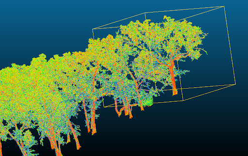
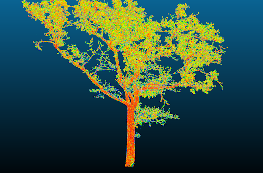
The project was presented to us by Dr.Lisa Bentley & her graduate student Breianne Forbes. Both are part of the Biology department. Lisa Bentley, Brieanne, and the rest of their team collected 3D images of the forest. Using a terrestrial laser scanner, which is a contact free measuring device, to collect dense point clouds of objects. In this case, point clouds are a set of data points in space that represent 3D objects. The figure on the left side is an example of multiple tree point clouds, while the image on the right is a single tree point cloud.
Machine Learning Approach:
The main objective was to classify forest attributes that are consired unclassified objects, like the ones below:
- Humans
- Tripods
- Low vegetation (Bushes)
- Trees

For this approach we wanted to employ machine learning to scan LiDAR files for trees. In order to create a machine learning model, we needed to have training data for LiDAR’s machine learning algorithm to digest. The toughest hurdle in this project was forming and collecting enough data to create a model that could consistently classify forest attributes, such as trees, bushes, humans, and the tripod that captures it all. Thankfully, LiDAR came with its own built in algorithm, we simply needed to make sure that our machine learning model was learning the correct way to classify forests. Many drafts of the model were made with slight modifications to the traning data. Initially, we used a plot of trees that did not have much diversity like no ground cover, shown in Figure A.
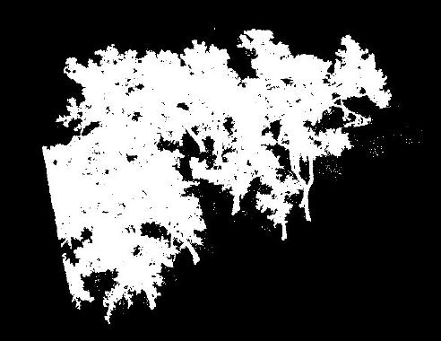
Figure A
Figure A is a view of our initial data set. If you look at the base of the trees, there is no ground cover for our algorithm to process. It was at this point in our project that we realized how we needed to compile our training data. Simply learning what a tree is will not be enough for our model to classify an object as a tree, if we do not include any ground cover. We then transitioned to using partitioned sections of large forest plots, seen in Figure B. The plots in Figure B all follow the same representation, with some variance. Namely, each plot has a tree, some bushes (classified as low vegetation), ground cover, with the possibility of having humans as well as the tripod. It is important to note that while they are similar to each other, they carry enough variance to keep our model from making simple assumptions. In our model, simple assumptions are our worst enemy. Our first model assumed that beyond a certain height, any points in our data were classified as tree points. In order to eliminate this, the usage of low vegetation plays an important role. Since low vegetation varies in height, our algorithm could no longer make the assumption that our first model made. The existence of more classifications within a plot forces the algorithm to search for a deeper understanding of the anatomy of a forest. In our case, using the training data in Figure B was effective in creating a complex model to accomplish this. Using this training data, our Machine Learning algorithm will look at the four subplots and determine how to classify the six classes denoted in the classification key.
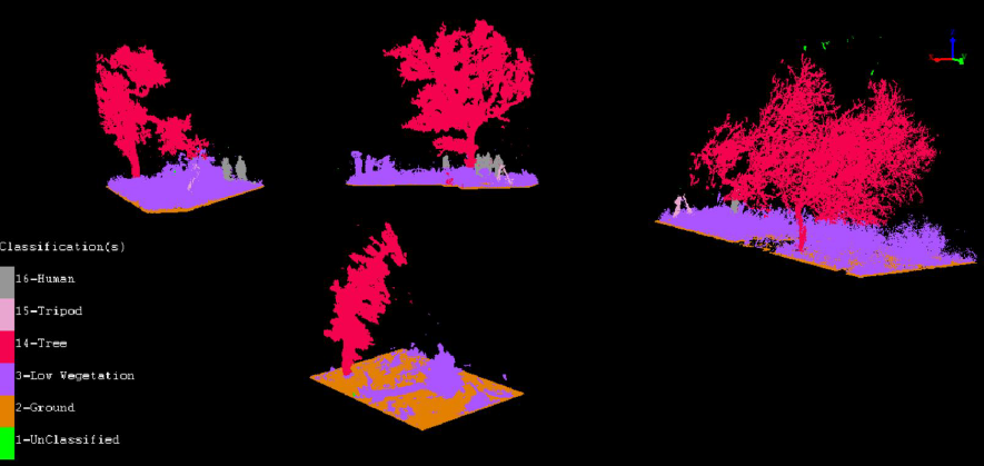
Figure B
Testing Our Trained Model:
After we trained our Machine Learning Model, we were able to test it on plots to see how it performed. Overall, we were happy with our results because we were able to identify more than just trees. Figure B above shows the different classifications we managed to obtain. Our model, could tell the difference between different objects in the forest, for example trees and humans. Below are some of our results we got from running our model. The figure with RGB colors is the original image and the one on the right is the output image we get after running our trained model. As you can see, we classified trees with a red color, purple for bushes, and what seem to be humans in a grey color. With that said, one issue we had was that we missclassified the humans legs as bushes.
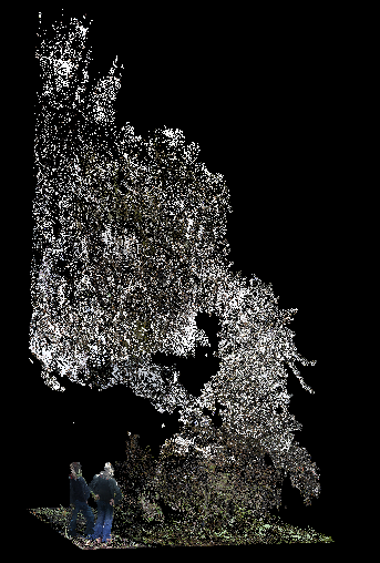
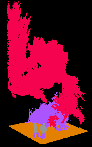
Figure C
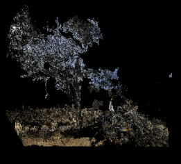
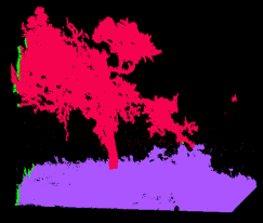
Figure D
Before the Machine Learning Model approach, in order for a tree to be measured, a Biologist would have to manually separate the trees in LiDAR. Also, biologist had to go out in the field and manually classify objects in the forest. With the usage of our work , we are able to reduce labor by automating the process of finding trees and other objects within LiDAR. While the training data we curated is more compact, practical forest plot files can easily reach over 10 GB. Once the forest is classfied into trees along side other objects, we go on to the next stage obtaining QSM parameters. For each tree plot we were given we applyed the second approach, which is articulated in the next paragraphs.
Python and Matlab To Construct QSMs:
Python and Matlab have a wide variety of tools to build QSMs from trees represented as point cloud data. Using pre existing modules such as Open3D for python and TreeQSM for Matlab, we were able to automate the process of creating the QSM objects for the trees.To start off, we created 3 scripts that encapsulate the creation of the QSM objects for each of the trees given to us. The first script would take the PLY files created by third party software and turn them into txt files that contain the [x, y, z] coordinates for each point. If the third party software can produce txt files, this part can be skipped. After the filtration process, the second script would then call on the Matlab modules to begin the creation of the QSM objects. The third script would check that all the requirements are installed on the host computer, create the needed directories, then begin the pipeline between the first two scripts to produce the final output. Once the QSM is constructed, we can extract the data contained inside. This method has a faster time complexity and increases the amount of ground covered compared to the traditional task of going out and taking measurements by hand.
Results:
Below is an example of the output we got when we ran our script of one of the trees as the input file. We managed to calculate different tree parameters as shown below. For example, we calculated the tree height and the total volume for tree p1301_1002.
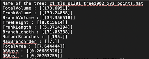
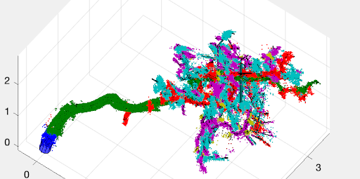
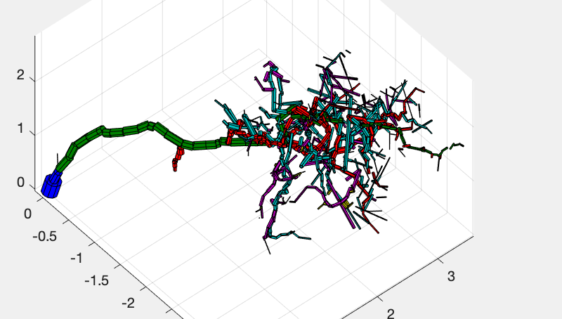
The table below compares the originally collected data with our results of the data recorded when we ran the script on 21 individual trees. Data collected by hand in the field is the originally collected data. Overall, the code worked well and it was very accurate in estimating tree parameters. The average difference overall was around 1.28cm for the DBH Height (Diameter at breast height).
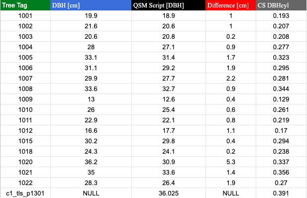
Eventhough we got good results there were a few discrepancies. For example, the QSM code dosen't seem to recognize trees with branching stems well. Any data we were unable to collect returned as NULL. As shown in the table below, the code missed one tree and created a non-existing tree. This can be fixed by improving and further developing the code.

Since the second method was not very machine learning oriented in itself, it required machine learning models or humans to give it the segmented trees for the QSM creation. This method could be added on top of machine learning models in order to create a completely automated process. Starting from the scanning of the landmass with the TLSR, to the eventual txt file that contains the data for each tree, or it can be kept as a stand alone script. Even though the scripts run as intended, there are some improvements that could be done to make it better. Due to the fact that matlab is needed to run the modules required to create the QSM objects, this would be a potential problem for many who don't have access to the Matlab program or can't afford a license. One solution would be to turn all the matlab code to python or another language that is more accessible to the public. Another possible improvement is to find ways to speed up the creation of the QSM objects through better usage of multithreaded operations. This being a clever and faster way of performing the mathematical operations given, that need to be done for most if not each of the points in the point cloud. The last improvement that could be implemented is to create a more user friendly interface, such as a GUI or some other kind of visually oriented form of interaction. Providing this level of abstraction would speed the process up for users.
Conclusion:
In conclusion, the forest is classified into trees, then trees are segmented, resulting with the QSM parameters being obtained. Using machine learning to classify unclassifed objects as trees, humans, and bushes will elimniate the need to physically be present in the forest to identify the objects. Second, using matlab and python scripts, we specify exactly which tree parameters we want to extract without having to physically mesaure it in the field. This allows for more time to spend on analyzing the data then on aquring the data out in the field. With the data collected, proper measurments can be taken to reduce wildfires. It can help detect forest that are prone to having a wildfire due to the forest enviroment been dead and dry.
Refrences:
Point Cloud Classification in LiDAR360
Classify by Machine Learning
TLS Forestry Analysis in LiDAR360
TreeQSM- Github Script
Optqsm
TLSeparation