CS 385 : Text Detection
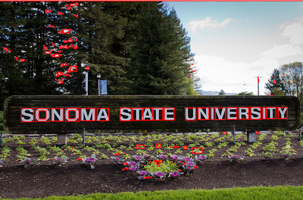
figure 1: Example of bounding boxes.
Introduction
The overall goal of this project was to detect text within natural images. One of the first strategies we came up with was to split this task into two parts. First, we had to figure out an algorithm that was able to find where individual characters were within a picture. For this step we chose to use bounding boxes in order to identify where enclosed objects, such as letters, were located within the picture. In order to make sure the algorithm was working correctly, we decided to use a simple data set of images with little to no background noise and obscurities before moving on to more difficult images. After we felt that we had achieved this initial goal, we decided to expand upon our algorithm to make it more proficient and work with any type of image, regardless of how much of the image was actual text and how much was background noise. Once we were able to find where our characters were located within an image, the task then became more complex. We then had to train our program how to recognize and classify the characters to define them. By applying the HOG method we were able to classify characters found within the bounding boxes in order to distinguish them from one another. This brought along greater challenges to our goal and we were faced with many obstacles throughout the process; However, it provided a greater functionality to our program to not only detect where characters were within an image, but to also give them meaning.
Approach/Algorithm
1. Bounding Boxes
One of the first methods we found was the use of bounding boxes. This method characterizes where a character is versus what is the background of an image and then creates a bounding box around each character (see figure 1). First we had to resize each image read in Matlab to be three times its original size in order to make it large enough for the characters to be recognized. Next, was the task of determining where text was in the image compared to what was just background. To do this we used edge detection techniques to isolate the background from the text. Initially the Prewitt and Sobel functions within Matlab proved to be the most effective when using a threshold of 0.5 and 0.09 respectively. However, after testing multiple images with these edge detectors, the Canny method proved to be the most
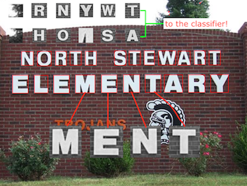
figure 2: some of the extracted bounding boxes sent to classifier.
bwareafilt and extracted the connected objects from the image within the range 500-5000. Some of the characters were lost in the initial edge detection stage due to minor edges being lost, that would enclose the character. In order to capture more enclosed characters, we used dilation to expand our found edges. Characters were the majority of the enclosed objects detected however, there were several enclosed/connected non-character objects in the background that were included in these extracted features which we took into account and resolved later using a classifier. After this step, we took the complement of the result and used regionprops to create bounding boxes around the objects found. We were then able to extract the objects within the bounding boxes and save them as individual images. These images were then passed to our classifier which was able to determine character versus non character objects (see figure 2).
2. HOG
im_crop. The classifier was trained to detect characteristics of every character, including uppercase letters and numbers. These learned classifications were compared to the characteristics of every object found within the bounding boxes. To detect these characteristics we decided to use the HOG (Histogram of Gradients) method. In order to implement this method we used several variables including:
Training Images : This variable set the correct path through folders to extract images' names.
Taining Boxes: A 4 X N array of object bounding boxes. 4 represents Xmin, Ymin, Xmax, and Ymax respectively. N represents the number of bounding boxes.
Training Box Image Names: A 1 X N list of the names of the images containing bounding boxes.
Training Box Labels: The object label for each bounding box.
Training Box Patches: A 64 X 64 X 3 X N array of patches for each object.
|
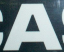
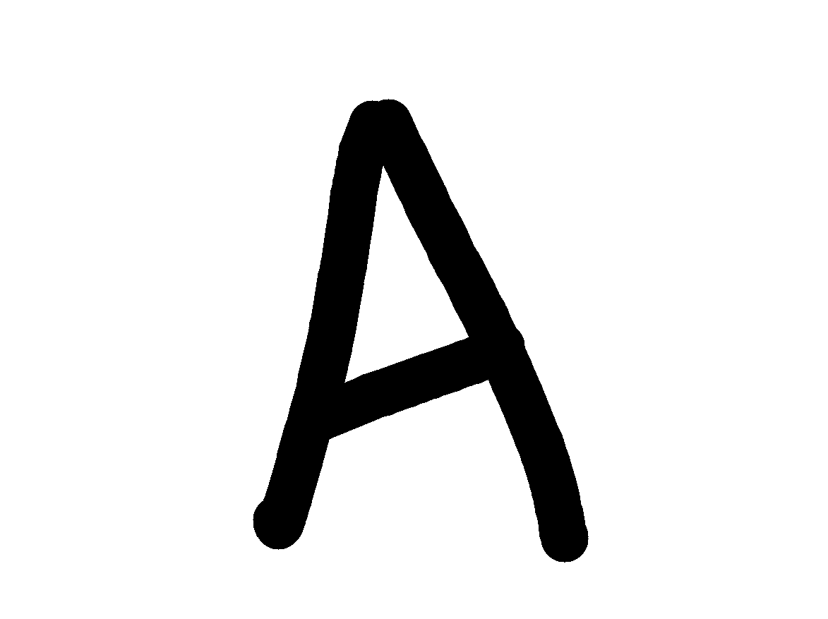
figure 3: Small example of positive data sets for 'A'.
vl_hog (These results can be seen in figures 4 and 5 below). Once the features of the character were defined, we were able to compare the images from the bounding boxes to this set of features in order to detect what the character within the bounding box was. This was computed by getting a score for the character to see how closely its characterists were related to the characterists found by our HOG function. First, we created an array of scores for the positive and negative images using vl_nnconv. By using this array with the ROC function, we got a threshold for our character (each character contained a different threshold). For example, our calculated threshold was determined to be 25.3115 for the letter A, meaning that if our extracted images score was below this threshold, we could be confident that it was not the character we compared it to, and we could move on to the next character until we found a score above the threshold, signifying a positive match.
We organized our data into separate folders with names corresponding to the index of an array containing all characters we are able to identify. We are able to identify 36 characters in total, including all 26 letters of the English alphabet and numbers 0-9. We then looped through all character files for our positive training data and stored the mean HOG feature map for each character to a cell in an array, each index mapping to their respective character from the data in our organized files. From there we were able to take individual images sent from all bounding boxes and compare them to each of the mean HOG maps. We then saved the score of the comparison to each of the maps in an array where the index also corresponded to the array of characters. We extracted the index of the maximum score from this array. If it passed the threshold for the character at that index we can be confident that the two characters were a positive match.
HOG Features
figure 4: Mean of the HOG features for the letter 'A' which we used for our classifier.

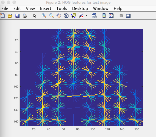
figure 5: HOG features for test image of 'A'
Results
We started out by testing our algorithm with individual images of characters against their respective correct matching character. We looped through a list of test images and compared these with the HOG features for that image. We repeated this process with images that did NOT match the character we were testing. If the score a character obtained was lower than the threshold it was compared to, we rejected it as being a match and added 1 to the correct guess score. This test was run through several different inputs of characters and overall we found that our positive and negative data sets had an average of a 97.22% accuracy in finding matching characters to their classifying HOG descriptor. We found that our classifier was sometimes confused by images that were very similar in features. For example characters such as 'c' and 'o' had very similar features and would sometimes be misclassified. However by choosing the character that gave the higher score matching to the HOG features, it overcame this obstacle. Through this testing we realized that it is not the quantity of testing data that returns the best results, rather it is the quality. If we had a lot of images that were not high quality, there would be more features added to the HOG classifier that were not useful. We also found there would be a higher acceptance rate and therefore less accurate threshold for characters when we had more input data. Finally, we found that when we used images for our input data that was more closely related to our testing data, we were able to detect features more accurately. Since we obtained our training data first, we had to search for input images that were faced more straight forward than tilted at an angle, with very little or preferably no illumination variation, occlusion, or deformation.
Overall, our project started out as simply being able to identify where text was located within an image and by the end we were able to identify what we were detecting with a very high accuracy rate.
Conclusions
We were faced with many challenges along our path to a final result. One of which was the use of edge detection to find characters did not seem to be as effective as it could have been. Perhaps a better approach would be to use the sliding window method. We probably would have extracted fewer non-character images from the background, and we would have been able to detect characters with more accuracy from the beginning. Some characters were left as unidentified within our bounding boxes due to challenges such as occlusion and lighting blocking the outline of the character from being seen as a connected object. We also faced a challenge with our algorithm running a comparison to the mean HOG maps for every character was extremely slow. This could perhaps be improved by writing functions to store the data from the mean HOG maps into one place that could be repeatedly called, instead of having to run the maps from scratch every time. Finally, it would be nice to also include the lowercase version of each character within our training data. We originally planned to do this, however since it was taking an extended amount of time to run the mean HOG maps for just the uppercase character data set, we decided to cut out lowercase letters from our training. However, we do still have the datasets for these characters if we did want to include them later. By taking out these letters, we were able to reduce our dataset by about 80,000 images. Finally, we would have liked to eventually implement whole word recognition rather than character recognition. This was an ambitious goal from the start and after facing too many obstacles with the subtask of character recognition, we ultimatley had to change our plan. However, we now have our character recognition working with a relativelty high rate of accuracy. Perhaps now that we have the backbone for implementing word recognition, we would be able to do so, given more time.
References
Campos, Teo, and Manik Varma. "The Chars74K Dataset." The Chars74K Image Dataset - Character Recognition in Natural Images. CVSSP/Surrey, n.d. Web. http://www.ee.surrey.ac.uk/CVSSP/demos/chars74k/.
Mallick, Satya. "Home." Learn OpenCV. Big Vision LLC, 06 Dec. 2016. Web. http://www.learnopencv.com/histogram-of-oriented-gradients/.
"Select Your Country." MATLAB Runtime - MATLAB Compiler - MATLAB and Simulink. MathWorks, n.d. Web.
https://www.mathworks.com/products/compiler/mcr.html.
Vedaldi, Andrea, and Andrew Zisserman. "Object Category Detection Practical." Category Detection Practical. Oxford Visual Geometry Group,
n.d. Web. http://www.robots.ox.ac.uk/~vgg/practicals/category-detection/#object-category-detection-practical.
"VLFeat.org." VLFeat - Tutorials HOG Features. VLFeat.org, n.d. Web. http://www.vlfeat.org/overview/hog.html.
Wang, Kai, and Serge Belongie. "Word Spotting in the Wild." Computer Vision – ECCV 2010 Lecture Notes in Computer Science (2010):
591-604. Web. http://vision.ucsd.edu/~kai/pubs/wang_eccv2010.pdf.
Wang, Kai, Boris Babenko, and Serge Belongie. "End-to-End Scene Text Recognition." (2011): n. pag. Department of Computer Science and
Engineering University of California, San Diego. Web. http://vision.ucsd.edu/~kai/pubs/wang_iccv2011.pdf.